Introduction
This tutorial provides an overview of BTField functionality for Advanced Geophysical Classification (AGC) of dynamic UltraTEM data. We will process a one-pass UltraTEM Portable Classifier data set collected at the Ramona Test Site (RATS), San Diego, California.
Good luck, and have fun!
Tutorial steps
Setup and data import
-
Download the BTField data and project, and processing flow files.
-
Load the BTField project. See the project import documentation for more details.
-
Create the site and import the data. See the data import documentation for more details
Tip: The name of your BTField site must match the name of the site that was used to collect the data. The site can be determined by the string preceding the ‘(‘ in the data folder name, in this case: RATS P 2Fa-hdf5 -
If this is a new installation of BTField, load the DoD library.
Preprocessing and target selection
-
Load and run the “P Flow1” processing flow. Note: right click on the f(x) button in order to access the option to load the flow. This flow removes data that does not meet positional MQOs and demedian filters the data.
Tip: If the Process button is not enabled for the P Flow1, double click on the production survey in the Site tab to select it. -
Now grid the data as shown here:
-
Create a new indicator with the filtered data by dragging the -a data state in the P1 flow to the Gridded Observations view
-
Right click on the indicator to configure it. Create a new time channel operation that sums all channels between 250 us and 500 us. We call this the “tearly” channel and it is most commonly used for target picking with UltraTEM data.
-
Configure the Tx-Rx pairs. Select each transmitter and then select the transmitters that are inside each transmitter to create the “Inclusive-Z” measurement pairs that is used for target selection.
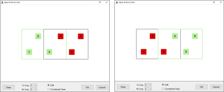
Configuration of Inclusive Z measurements. -
-
Configure a target picking function to pick targets at 5x the noise. See target picking documentation for more details. Recommended target picking parameters are shown below:
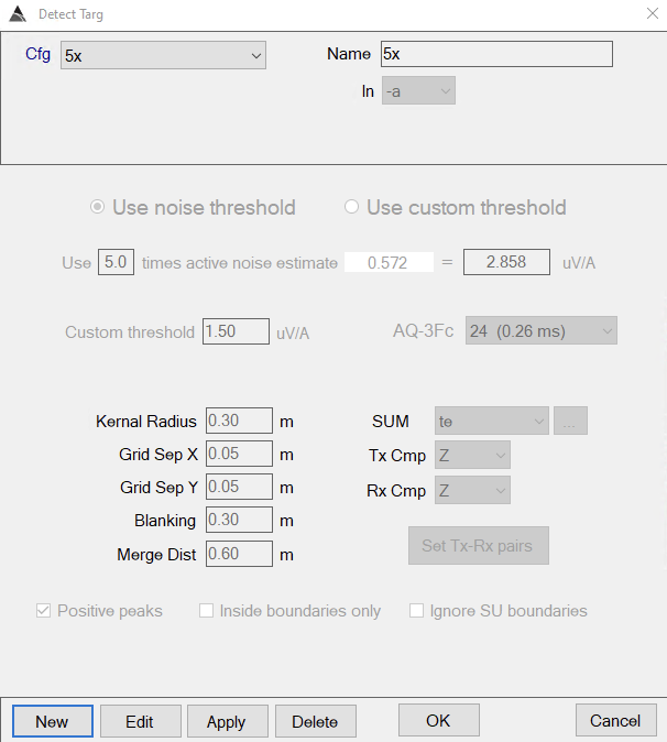
BTField picking configuration. Picking threshold will vary slightly depending on your noise polygon. -
Now define a noise polygon by delineating an anomaly-free area in the data. Once this is defined, run the picking flow by clicking “Auto-pick”
Inversion and quality control
-
Invert the targets.
- Create cells
- Set up and run the inversion. See images below for recommended inversion parameters and inversion mask
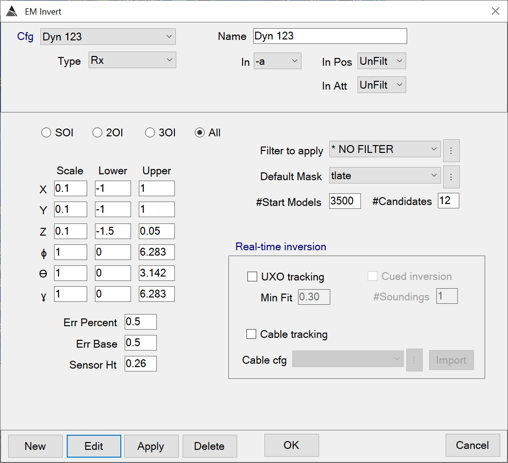
Recommended BTField inversion configuration. 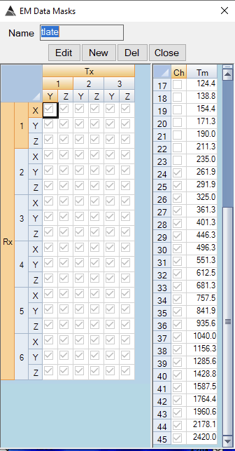
Recommended BTField inversion mask: invert using all transmitter-receiver combinations and all time channels from 262 microseconds onwards. -
QC the inversions by:
- Resetting the status of all targets. This ensures that the dig list will give consistent results when it is re-run.
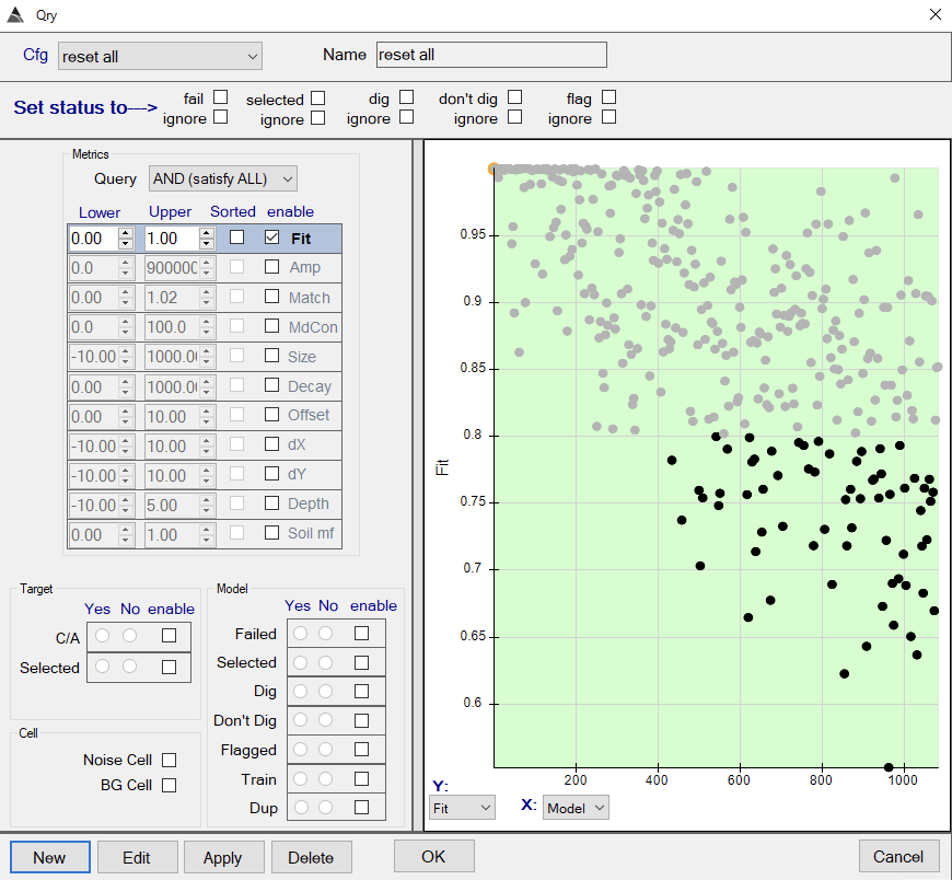
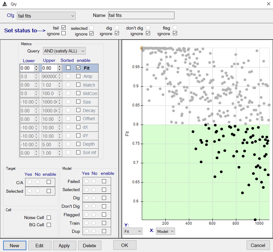
BTField configuration for resetting the dig list. - Failing inversions that have data fit less than 0.8
BTField configuration for failing inversions with data fit less than 0.8. - Failing models at inversion bounds. The queries for horizontal offsets (dX and dY) shown below will fail models with either positive or negative offsets from the pick location.
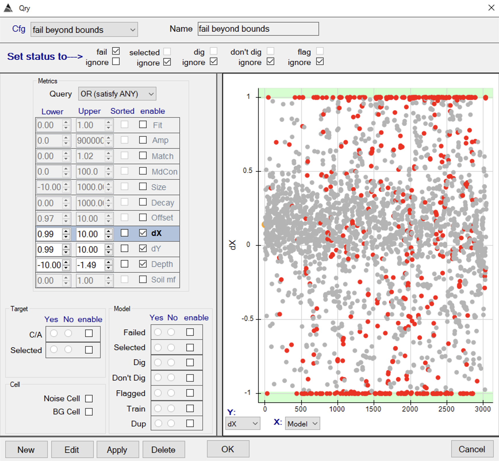
BTField configuration for failing models at inversion bounds.
Classification
-
Set up the first stage of classification using all polarizabilities:
-
Configure the site specific library for this stage. The following items should be included in the library. Use only the Mark/Mod indicated in brackets where given, otherwise use all available variants in the DoD library:
- 155mm Projectile
- 25-lb bomb
- 2.25-in rocket
- 2.36-in rocket
- 2.75in Rocket
- 37mm Projectile
- 60mm Mortar
- 75mm Projectile
- 81mm Mortar (M821)
- 90mm Projectile
- Hand Grenade (M30, M30/M62)
- Rifle Grenade
- Large ISO
- Medium ISO
- Small ISO
-
A “Metrics view” is required to run tlshe classification. To enable this view, right click on an existing view, split the existing view (if desired), and then right click again and set the view to “Metrics View.”
-
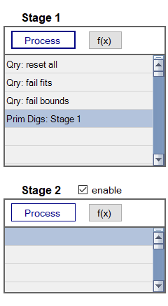
Enable the second classification stage so that your classification processing flow is as shown below. Stage 2 should be enabled so that you can specify a “lock point” at which the dig list will switches between the first classification stage using all polarizabilities and a second stage using a primary polarizability match that we will configure later.
Set up of stage 1 classification flow. -
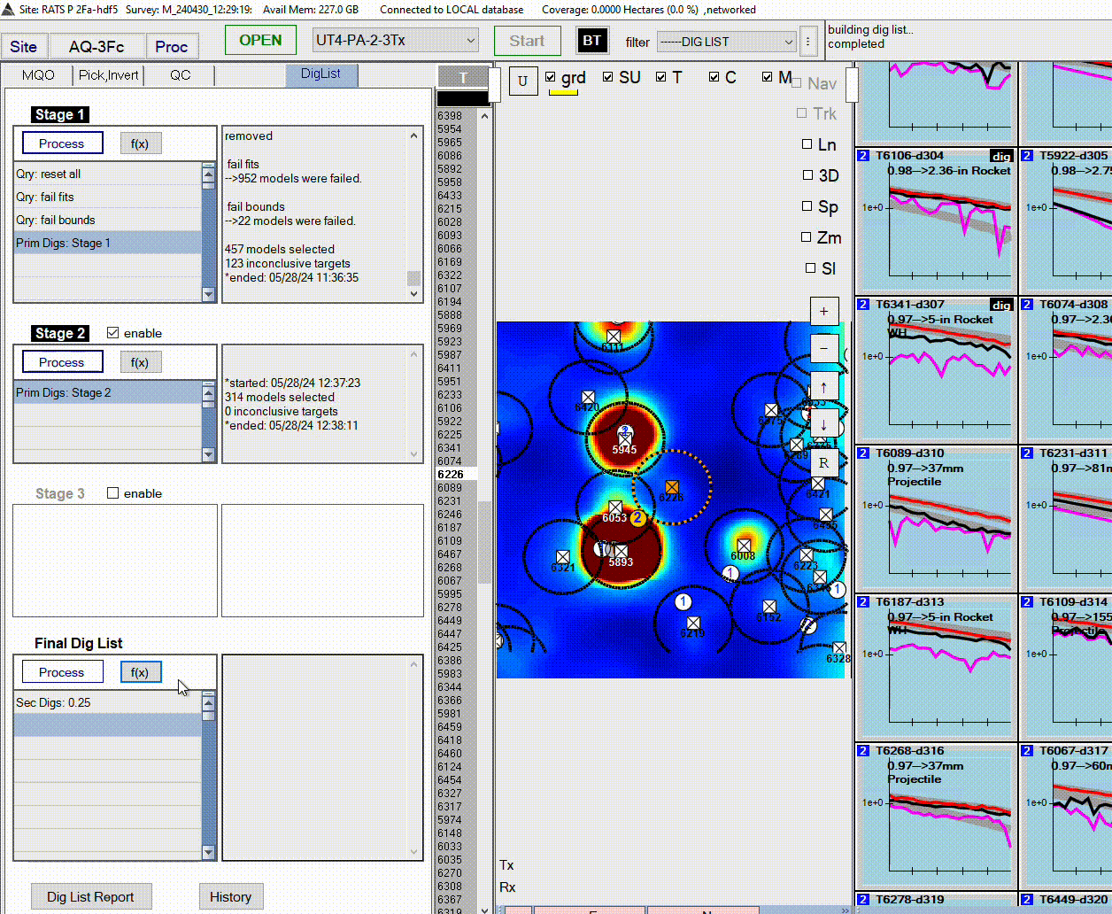
Run the first stage by clicking the blue “Process” button for Stage 1. You should now see a ranking of targets by polarizability match. Each subplot in the dig list order shows the match between predicted polarizabilities and the best matching library item:
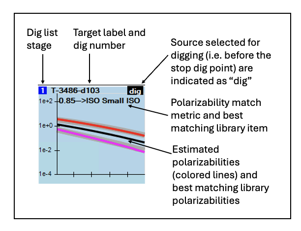
Layout of polarizability plot in the dig list. Tip: The polarizability match metric is calculated such that 1 indicates a perfect match to the library. Targets are ranked in the dig list by decreasing polarizability match.Plots in the dig list are colored by category. At this stage of the process you will only see Inconclusive and Primary Dig categories:
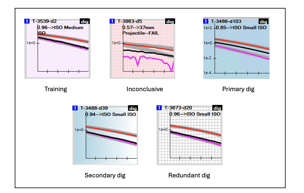
Plot backgrounds in BTField dig list. Tip: You can reload your dig list at any point (e.g. after restarting BTField) by activating the dig list filter. Click on the dropdown to the right of the black BT button and select DIG LIST -
Select a lock point by reviewing the stage one dig order and selecting the last target giving a good match to the library using all three polarizabilities. To set the lock point, right click on the target polarizabilities in the ordered dig list view and click on “Stage 1 Lock”:
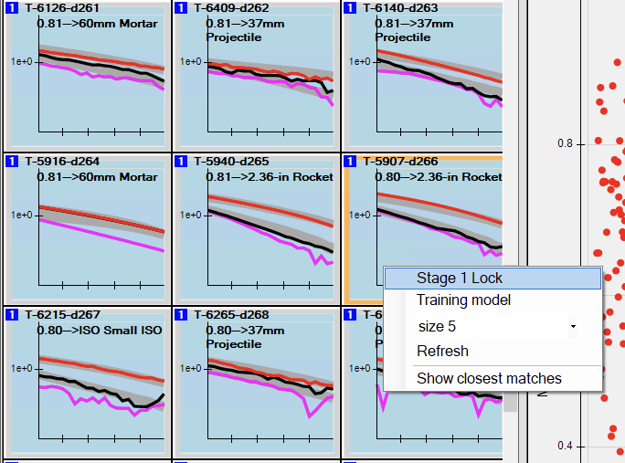
Setting the stage 1 lock point. The lock point should be set based on review of your dig list - the selected target in this image is shown for illustration only. Tip: Multiple classification stages are not always required. A primary polarizability match stage is used here to identify vertically-oriented seeds that have poorly constrained secondary polarizabilties. Multiple stages may also be used to classify targets with different library configurations at each stage. -
Now configure stage 2 as shown here:
-
Add a primary dig function to stage 2.
-
Copy the library from stage 1 to stage 2, and then rename the copied library and set the match mode to “L1” so that only the primary polarizability is used for matching.
-
-
Run the second stage by clicking the blue “Process” button for Stage 2. The plot of polarizability match versus selected model index will now show a discontinuity where the dig list switches between stages:
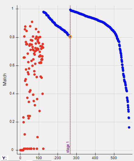
Polarizability in dig list order for the two stage dig list. You can click on points in this plot to navigate the dig list. -
Select a stop dig point by reviewing the stage two dig order and selecting the last target giving a good match to the library primary polarizabilities. To set the stop dig point, right click on the target polarizabilities in the ordered dig list view and click on “Stop Dig”:
Setting the stop dig point. The stop dig point should be set based on review of your dig list - the selected target in this image is shown for illustration only. -
Configure and run the final dig list flow:
-
Identify secondary digs. These are sources greater than a specified distance d (usually 0.25 m) from sources already selected as digs. The secondary sources also meet the criteria to be classified as a target of interest in the dig list. This step is required in order to identify cases where inversion of a single target pick estimates multiple unique sources (separated by at least d) that should be dug.
-
Identify duplicate digs. Multi-object inversion can produce many redundant sources estimated for each physical object in the ground. To generate a set of unique source locations for intrusive investigation, we merge sources together using a specified horizontal merging distance (usually 0.25 m). If two sources are within the merging distance of each other, the source that is ranked highest on the diglist will be retained on the final listing of unique sources.
-
-
Export your dig list by clicking on the “Dig List Report” button. When prompted, select “TEST” as the Type for the report. Additional fields for the report can be left blank.
Score your diglist
Check your diglist performance by uploading the xlsx dig list exported from excel, then click on the “Score dig list” button: