Configuring Post-Processing Flows
Once data has been collected, it has been processed by the Real-Time flow. All Real-Time flows have a Merge function labelled RawMerged, therefore, at a minimum, the collected data will be merged to the time base of the EM sensors. If the Detrend function was also included in the real-time flow, the data would be considered “processed” and immediately ready for inclusion in a Master survey where target picking and inversions are typically performed. However, if the Detrend function was not used in the real-time flow, a post-processing flow would be required to detrend the data.
There are six post-processing flows available:
-
P Flow1: used for auto-processing single surveys on import, and for batch processing.
-
P Flow2: An additional flow for processing single surveys.
-
P Flow3: An additional flow for processing single surveys.
-
M,SU Flow1: used for auto-inverting master surveys after target picking.
-
M,SU Flow2: An additional flow for processing master surveys.
-
M,SU Flow3: An additional flow for processing master surveys.
For example, we can configure the P Flow1 flow by clicking the f(x) button and dragging in the Detrend function to prepare the data for inversions:
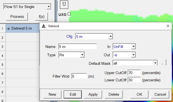
Now any single survey can be loaded and detrended by clicking the
Process button.
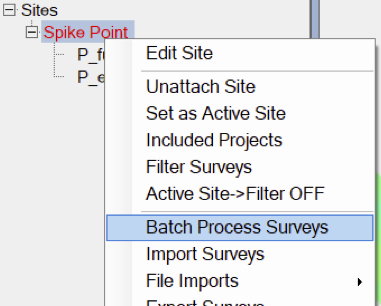
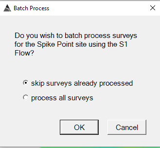
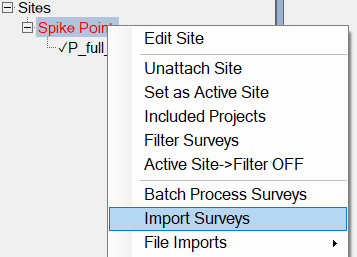
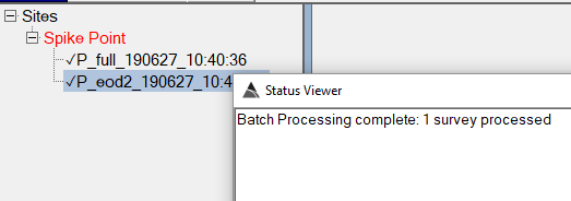
Batch Processing Surveys
All Production surveys can be processed at once by the S1 for Single flow by right clicking on the Site and selecting “Batch Process Surveys”. The user has the option of processing or (re-processing) all surveys, or skipping surveys already processed:
 |
 |
|---|
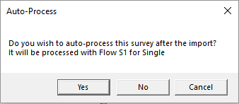
The user also has the option to run the P Flow1 flow during
import of a survey(s):
 |
 |
|---|
After the survey(s) have been processed, a check mark will appear in
front of the survey name to indicate it is ready for inclusion in a
Master Survey:
Creating a Master Survey
To pick targets and invert data collected across multiple surveys within a site, a user can create a Master survey for the site. Right click on the site’s name and select Create Master as shown. The Master survey will load and display all processed (detrended) surveys for the site
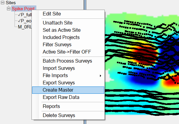
As new surveys are added to the site, the Master survey will
automatically update itself. Target picking and inversion can now be
performed while having access to all historical data collected over
each anomaly.
Picking Targets
Targets can be picked in either a Single Survey or in the Master Survey. It is recommended to pick targets in the Master Survey since it allows the user to visualize all historical data collected over the anomaly. To pick targets, an Inversion Results View must be added (see Section 5 – Configuring Your Machine’s Display Views). With the Master Survey loaded, click on the Start Picker button in the Inversion Results View:
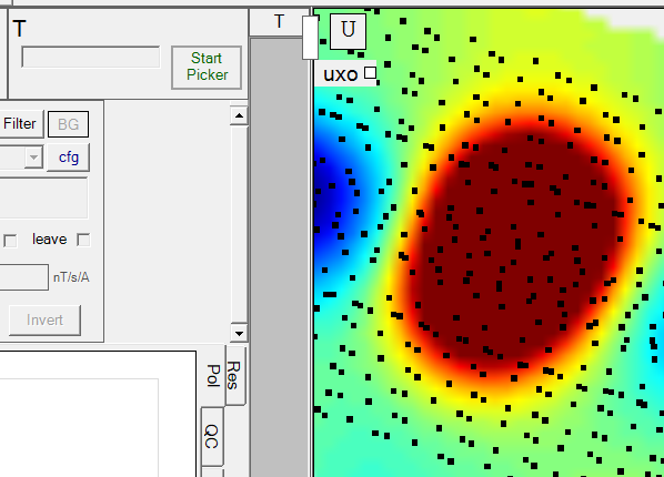
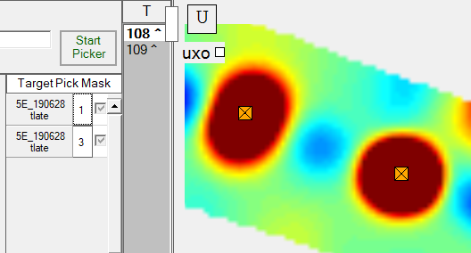
Once the Picker is started, it will display the single surveys and
line numbers found within the currently zoomed area. Pressing the X
key while left-clicking will pick the target:
 |
 |
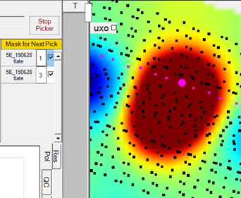
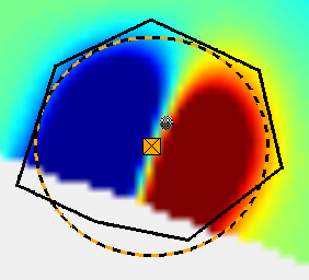
If desired, specific lines can be unchecked to achieve the optimal visualization of the data to be inverted. For example, line 3 can be unchecked to visualize the gridded Y component:
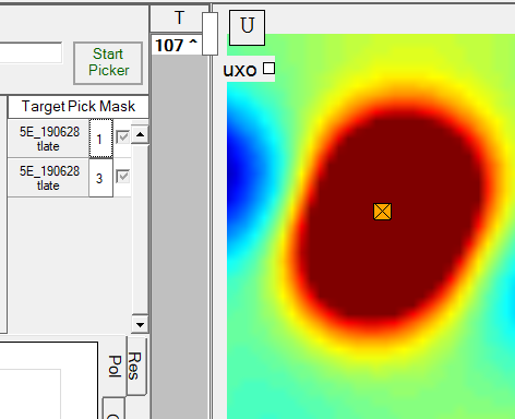
Once the target is picked, it will retain the visualization that was
used for the pick decision. The Picker can be started again at any
time to continue picking more targets:
Inverting Data
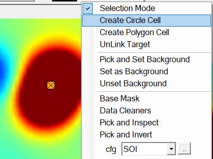
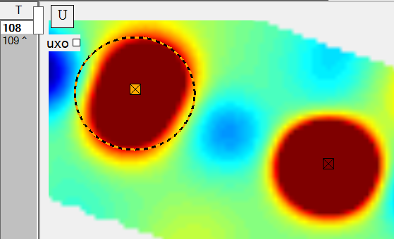
To invert data around a target pick, a cell must be created first. Cells can be circular, or polygon shaped. For example, a circular cell can be created around the target 108 by right clicking and choosing “Create Circle Cell” from the menu. Click, hold, and drag out to display the circular cell, then release to create it:
Note that target 108 now has its hat (^) symbol removed in the
target list, indicating that it is now associated with a cell:
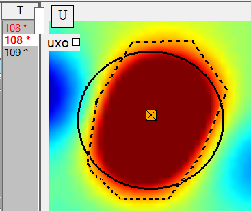
To create a polygon cell, select “Create Polygon Cell” from the
menu, click successive points, then press Enter to close the polygon.
Note that in our example, target 108 now has two cells associated with
it. The red color in the target list indicates that a decision will be
required to select the cell with the best inversion results:
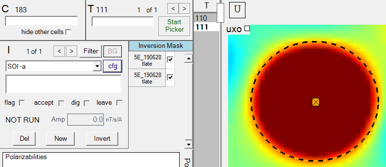
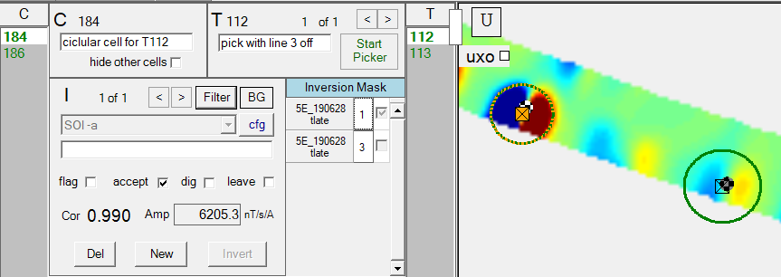
Once the cell is created, the user can invert the data within it by
clicking the Invert button. The inversion will proceed using the
currently selected Inversion configuration. For example, in the
screenshot below, the “SOI -a” inversion configuration will be
used when the user clicks the Invert button (SOI stands for Single
Object Inversion). The settings of the inversion configuration can be
accessed using the blue “cfg” button.
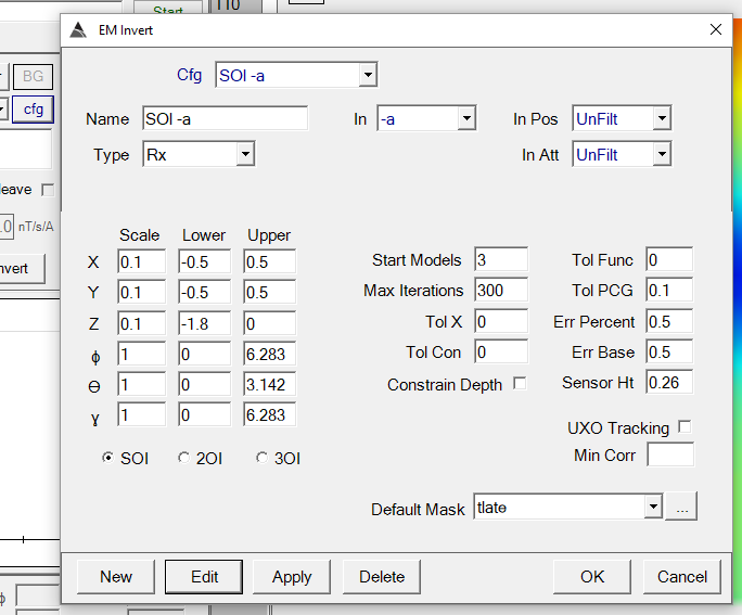
If we click on the cfg button, we can inspect the SOI -a
inversion configuration as shown below. It accepts the detrended
-a data state as the In parameter, while using the unfiltered
data states of position (In Pos) and attitude (In Att). The
horizontal bounds are set to constrain the xy fit location to within
+/- 1.0 m from the target pick location. The vertical fit location is
constrained to be between ground level and -1.5 m. The sensor height
is set to 0.26 m, which was the platform height above ground during
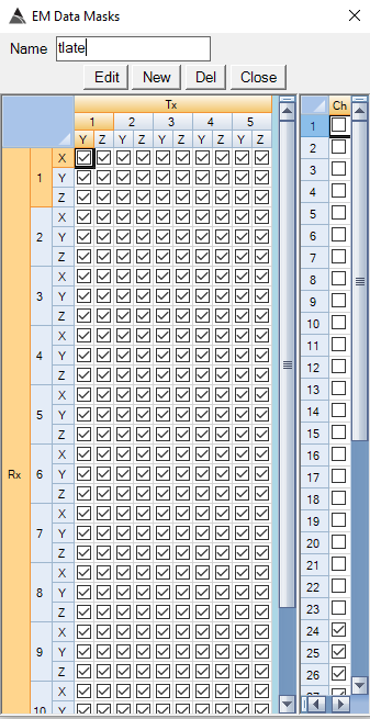
collection. The Default Mask is tg24, which has only the late
time channels selected (gates 24 to 45). When a new cell is created,
the data masks for all lines falling within the cell will default to
use tg24.
 |
 |
|---|
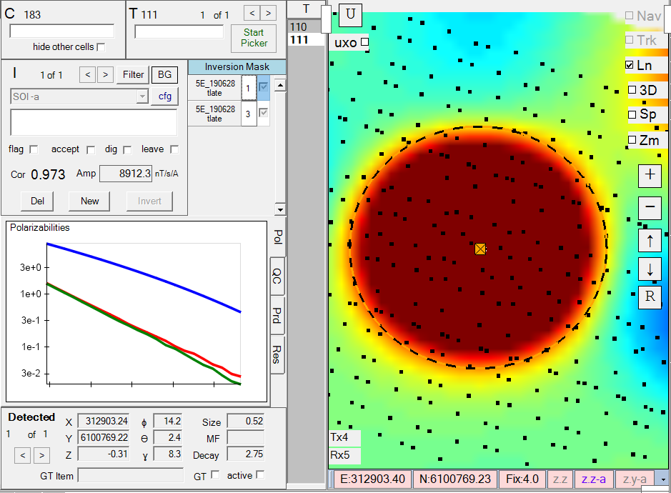
Once an inversion configuration is created, any cell can be inverted by clicking the New button to create a blank inversion for cell. The Invert button can then be clicked to invert the cell data. The inversion results will be immediately displayed as shown here on the left side:
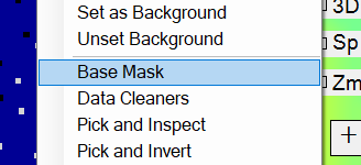
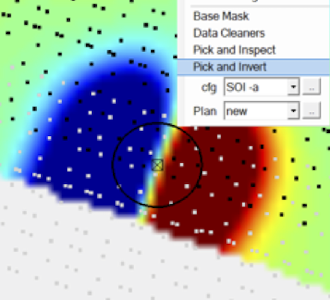
The user also has the option to pick a target, create a cell, and
perform the inversion in one step using the Pick and Invert tool.
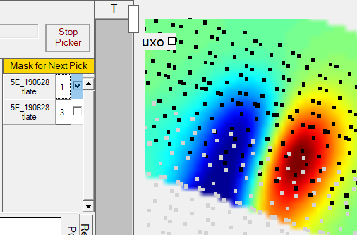
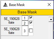
In the example below, the user has decided to first mask out an
unwanted line using the Base Mask, which is available off the
right click on the Grid View as shown here:
 |
 |
|---|
Next, they select the Pick and Invert tool from the menu and click, hold, drag out and release to perform all three operations at once:
 |
 |
|---|
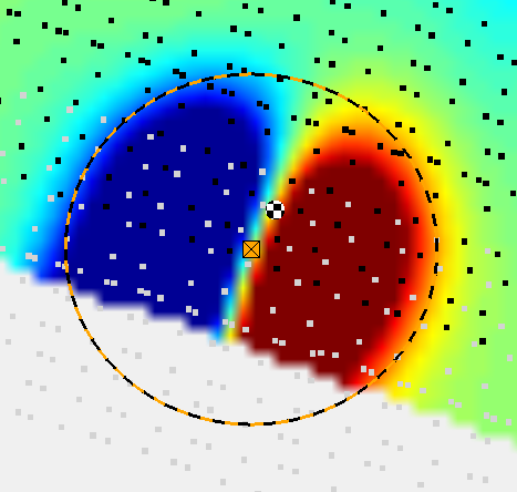
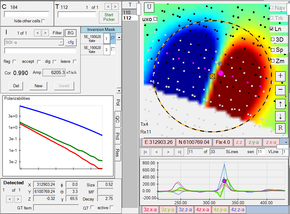
As soon as the user releases the mouse button, the data within the cell will be inverted. The detected location will show on the grid as a black and white checkered ball. Here are the results, showing a 9.90 correlation fit to the dipole model and the three principal axis polarizabilities of the item:
Batch Inverting Surveys
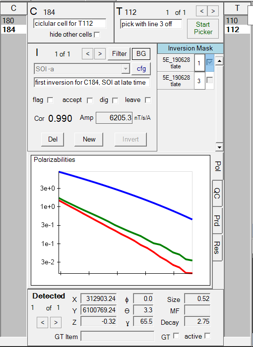
| A user may want to pick several targets first before inverting data. In this case it can be helpful to use the M1 for Master flow to automatically create circular cells around each target and auto-invert the data. For example, on the right is the M1 for Master flow set with Auto-create Cells using a radius of 0.5 meters, followed by an inversion that uses the EM Invert SOI inversion configuration. | 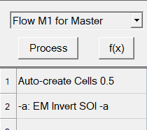 |
The user can run the flow at any time to invert recently picked targets. Therefore, a user can pick some targets, run the flow to batch invert and inspect results, then pick more targets, etc.
Analyzing Inversion Results
The Inversion Results view displays all calculated values from the inversion operation, including gridded views of the predicted and residual that provides immediate comparison to the observed data on the Grid View. For example, in the screenshot below Cell 2502 was inverted using the SOI inversion configuration which uses the late time channels as specified in the tlate mask. This inversion was performed with line 40 turned off, and it is the first inversion for Cell 2502. The inversion is showing a high 1.00 data fit (Fit) to the dipole model. In the Polariz tab, the principal axis polarizability (red) response is higher than the two similar transverse principal axis polarizabilities (black and magenta). This indicates the item has one long dimension and is symmetric about the other two dimensions (i.e. consistent with a uxo shape or metal rod).
The amplitude (A) is a summation of the inverted EM
observations. The value of 826.9.5 uV/A is taken from the Tx/Rx pair
having the maximum summation. Note that the Amp measure is dependent
on the inverted time channels, therefore cells must be inverted with
the same inversion mask to allow accurate comparison of amplitude between
items.
The predicted XYZ location of the item is displayed in meters. The X and Y values are represented in Easting and Northing, while the Z value is the depth below the surface. The best fit orientation of the item is shown using the angles of azimuth φ , dip ϴ, and rotation ɣ. In our example below, azimuth = 1.4 degrees and dip = 82.5 degrees, indicating the long axis of the item is almost horizontal and aligned to UTM north. The rotation about the long axis is 0.0 degrees.
If the Data Fit is sufficiently high (above 0.80), the Size can also be valuable for determining the presence of uxo. If only larger items are of interest, the Size measure can be used as a threshold. Note that the Size measure is dependent on the inverted time channels, therefore cells must be inverted with the same inversion mask to allow accurate comparison of Size between items.
If the Data Fit is sufficiently high (above 0.80 ), the Decay can also be valuable for determining the presence of uxo. Most uxo will have slow decaying polarizabilities that extend into late time before dropping off to near zero. Some users will see this immediately by examining the polarizability curves, but it will also be quantified by the Decay measure, which will typically be lower for uxo items.
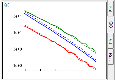
The QC tab Inv button (shown below) displays a gridded view of the predicted data, using the visualization settings of the currently selected Grid View indicator. This allows for easy comparison to the observed data in the Grid View.
It also provides a visual comparison between the decays of the observed data (solid lines) and fitted (dashed lines) data. Any location within the cell can be selected to display these decay plots for a specific Tx/Rx pair.
Creating and Using a Munitions Library
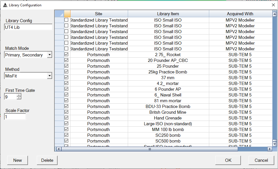
In the Inversion Results window, any inverted item can be marked as a ground truth (GT) item. This will make it immediately available for inclusion in a munitions library. In the Project Settings window, a munitions library can be created by selecting any number of ground truth items that may be present at the survey site. Below is an example of a library named UT4 Lib that was configured by selecting GT items collected at the Portsmouth site. The Match Mode can be set to match all polarizabilities, or just primary and secondary, or primary only. In our example here we have chosen to match the primary and secondary polarizabilities. The selected GT items were all inverted using time channels 9 to 45, therefore the First Time Gate must be set to 9.
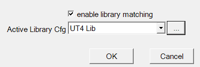
After setting the library configuration, we can enable it as shown here in Project Settings:
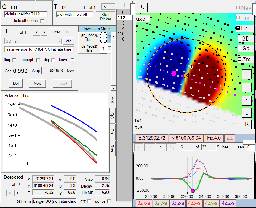
Now the all inversions for this BTField project will display the best match to the items in the active library. Below, our inverted example is indicating the best match is a Large ISO item with a library misfit (Lib MF) of 6.93. The library polarizabilities are plotted in grey for visual comparison to the inverted polarizabilities. Recall that our library configuration has its Match Mode set to “Primary, Secondary”, therefore only 2 grey lines are displayed. Also recall that the First Time Gate of all the selected library items is 9, but we are only inverting the late time gates (24 – 45). The plot automatically aligns the polarizabilities to their proper time ranges.
Setting QC Status and Filtering Inversion Results
In the Inversion Results view, there are four QC status states: flag, accept, dig, and leave.
A flag checkmark indicates a potential uxo item. This means the current inversion results are good enough warrant further investigation/analysis.
An accept checkmark indicates a detected uxo item. The inversion analysis of the anomaly has been concluded and the inversion results support a decision to classify the anomaly as a uxo. When a user checks accept, all other cells and inversions associated with the target will automatically hide, and the accepted cell with turn green as shown here:
 |
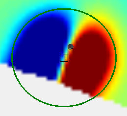 |
|---|
The dig check indicates the item should be excavated and removed.
The leave check indicates that although item has been flagged or accepted, a decision has been made to leave the item in place. This decision is sometimes made when excavation and/or removal of the item is unsafe, and leaving it in place is the safer option.
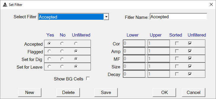
Filters can also be applied to sort on QC status and inversion results. Click the Filter button in the Inversion Results window to select or create a filter. For example, the “Accepted” filter is selected below:
After clicking OK, the Cell and Target lists, and Grid View, will show only accepted cells and inversions
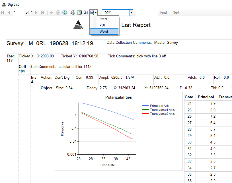
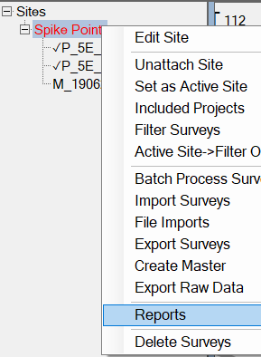
Generating Reports
To generate a report, a Master survey must have been created for the site. Right click on the site and select Reports:
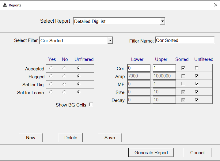
The Reports dialog will show, allowing you to select a report and optionally apply filters. For example, the Detailed DigList report can be selected and generated using a filter that will sort the items in descending order of correlation:
The report will be generated on screen, and it can then be exported to Excel, PDF, or Word using the drop down list shown here at the top of the report: