BTField user guide

Edit me

BTField User Guide

Version 12

A Single Solution for UXO Detection and Classification

Overview

BTField is a real-time data acquisition and classification system for unexploded ordnance. It has been designed to meet the needs of both data collection crews and geophysicists by allowing processing and inversions to run simultaneously as data is being collected. It is a 64-bit, networkable solution that can be flexibly configured to consume sensor data from multiple COM and/or TCP streams. Multiple users can establish a connection to the BTField SQL Server database and work in either a real-time acquisition and processing mode, or a post-processing mode. The SQL Server database is highly scalable, allowing for the attachment of multiple storage drives to hold significant volumes of geophysical data that can be queried and re-processed with different settings if desired.

Software Installation

First time installation

When BTField is installed for the first time, it will also install a SQL Server database. Therefore, the first msi installation file is much larger than any subsequent upgrade msi file.

After installing the msi file, run BTField. You will receive a message saying that it’s preparing BTField for first time use. This will take about 10-15 minutes.
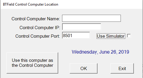
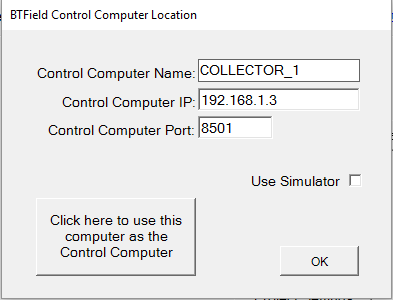
Once that’s finished, run BTField again, and it will prompt you for the Control Computer location:
Click on the button that says, “Use this computer as the Control Computer”. If you are going to use the Simulator, make sure the “Use Simulator” checkbox is checked. Leave it unchecked if you’re going to hook up to the actual sensors.
Click OK and it will prompt for your permission to do a few things in the background, and then it will exit.
Now you can run BTField.

Upgrades

An upgrade can only be run if the SQL Server database has already been installed by the first time installation.

Run the msi upgrade.
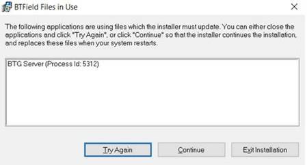
During the install it needs to upgrade the BTG service, which is always running in the background, so it will show this message indicating that some files are in use:
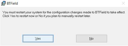
Click on the Continue button. It will then ask you to restart your machine.
Click on the Yes button to restart.

Single Machine configuration

If you only have one BTField installation, your machine will always act as the Control Machine. The Control Machine hosts the database and controls the Start and Stop for all data acquisition. When you run BTField, click on the button that says, “Use this computer as the Control Computer”. If you are going to use the Simulator, make sure the “Use Simulator” checkbox is checked. Leave it unchecked if you are going to hook up to the actual sensors.

Networked configuration

If you have two or more BTField installations on your network, you will likely want to select one as the Control Machine that runs the central database, then connect all other machines to it. The networked configuration is effective for both real-time data acquisition/processing, and post-processing.

When running BTField on the Control Computer, click on the button that says, “Use this computer as the Control Computer”. Leave the Control Computer Port on the default 8501.
When running BTField on one of the other machines (client machine), type in the Control Computer Name, and Control Computer IP. Leave the Control Computer Port on the default 8501.

BTField Projects

A BTField project defines a sensor platform configuration as well as the data parsing logic that consumes the sensor data. All processing is performed within the BTField project also. In the DAQ tab, there are four levels of parsing logic that extract the data – the Input level, Message level, Sensor level, and Data Extraction level. For example, the sample BTG Demo project shown below has a DAQ configured with one Input called Dynamic EM Stream, and it encapsulates two messages named GGA Msg and EM Msg. Each of these messages may contain data from one or more sensors such as a position sensor (POS), or several EM receivers (Rx) as shown here:

Typically, Black Tusk Geophysics will pre-configure these 4 levels of data parsing logic, but we discuss this example here to illustrate BTField’s flexibility to be re-configured in the field if necessary.

Data Inputs

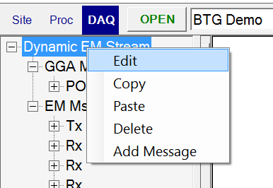
A Data Input is a stream of sensor data coming from either a serial COM port, or a TCP port. In our BTG Demo project, we can right click on the Dynamic EM Stream and select Edit:

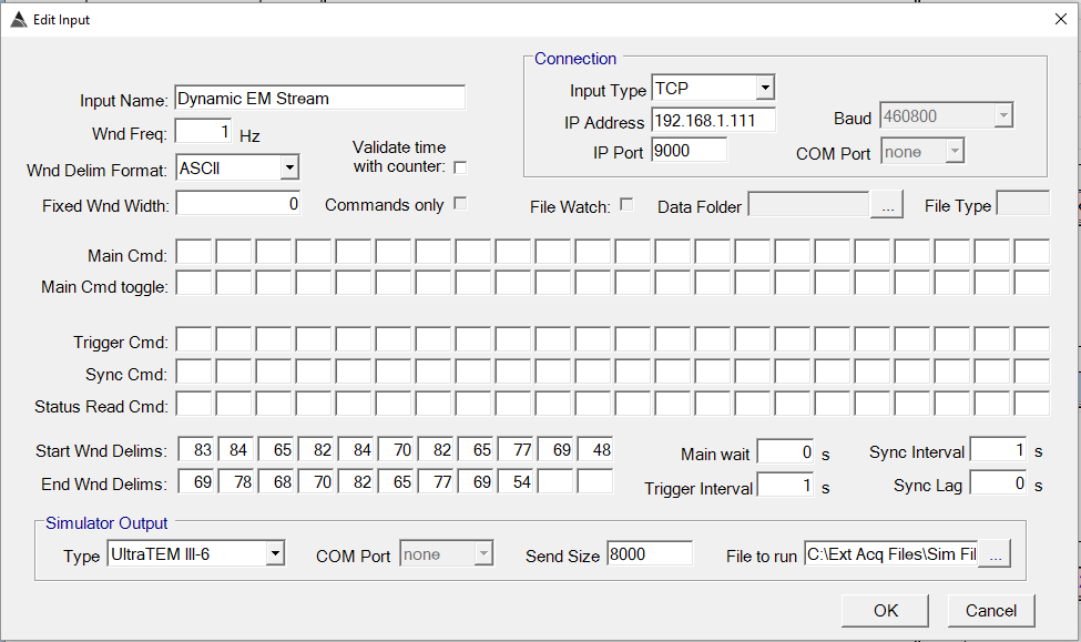
Here we can see it is a TCP stream that BTField will connect to at the IP address 192.168.1.111 on port 9000. The Start and End delimiters are also defined for one full data window.

Data Messages

An input definition will grab a full window of data from the stream. Within this data window, there can be several messages. For example, we can right click on the EM Msg message and select Edit:

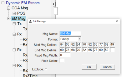
We can see this message contains Binary data that gets pulled out of data window using the specified start and end delimiters.

Sensor Definitions

A message may contain data from one or more sensors. Therefore, several sensor definitions can be established off each message node on the DAQ tree view. For example, we can right click on the first Rx sensor and select Edit:

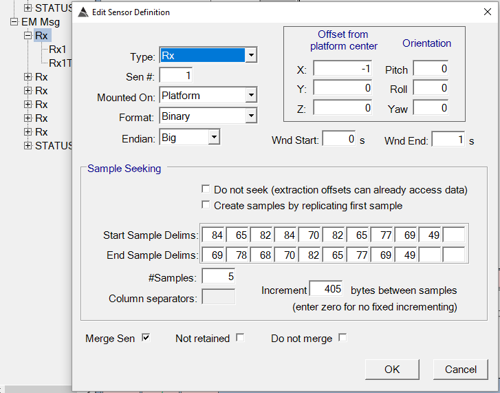
Here we can specify its Sensor #, its xyz offset from the GPS, and the parsing settings. We specify there are 5 samples of Binary Rx data and each sample is 405 bytes in length. We also check the Merge Sen checkbox to indicate we want to merge data to the time base of this sensor.

Data Extractions

The data for each sensor definition will contain the final readings that we want to extract and map to BTField’s data types. For example, we can right click on the Rx1 Data Extraction and select Edit:

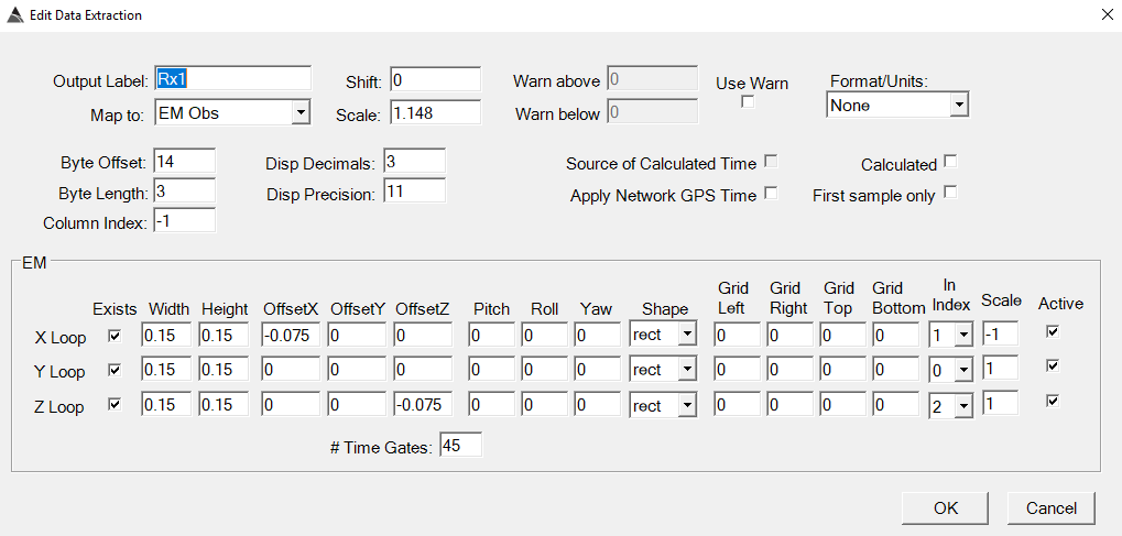
We can see it is mapped to the EM Obs data type, and we have also specified the loop geometry and number of Time Gates. The Byte Offset to the start of this sensor’s data is 14 and each reading has Byte Length of 3 bytes (i.e. a 24-bit number).

This is just one example of how data parsing logic can be configured in BTField. The 4 levels of encapsulated parsing logic (i.e. Inputs, Messages, Sensors, and Data Extractions) can be configured in numerous ways to provide a flexible means of consuming data from a variety of different sources and formats without the need for additional programming.

Loop Geometry

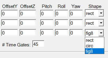
Loop geometry is also set in the Extraction window. The OffsetX, OffsetY, and OffsetZ are all relative to the parent Sensor definition that established the center position of the loop. The loop Width, Height and Shape are also set in the Extraction window. Three different loop shapes can be specified – rectangular, circular, and figure 8:

Sensor Commands

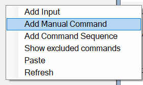
Sensor commands can be added in the DAQ tab to control sensor output directly from BTField via TCP or serial. Right click in the DAQ tab and select Add Manual Command.

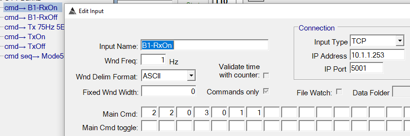
Here is an example of a command named B1-RxOn, which turns on all platform receivers via TCP by sending out the bytes 2 2 2 0 3 0 1 1 (decimal format):

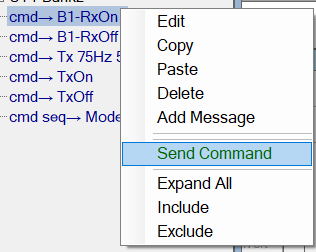
The command can then be sent manually by right clicking on it and selecting Send Command as shown:

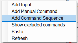
Commands can also be sequenced together and sent all at once by selecting Add Command Sequence:

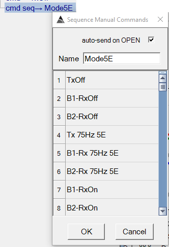
Here is an example command sequence that will turn off all transmitters and receivers, set the frequency, then turn all transmitters and receivers back on. Note the user has checked auto-send on OPEN, therefore BTField will always send this command sequence when a survey is first opened:

Configuring the Real-Time Flow

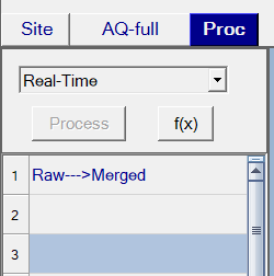
When BTField begins collecting data, it will execute the functions specified in the Real-Time flow found in the Proc tab. The Real-Time flow has one Merge function by default. This function is responsible for merging all raw data to the time base of the EM Sensors.

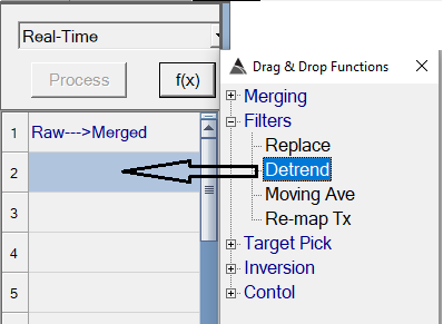
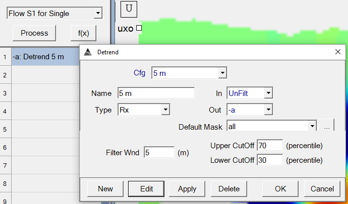
More functions can be added to the flow by clicking the f(x) button to display the Functions dialog. For example, the user can drag and drop the Detrend function into step 2 of the flow:

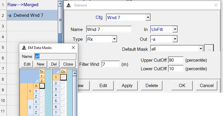
After dragging it into the flow, its parameter settings dialog will pop up. The Detrend function removes large geophysical trends and prepares the data for inversion. We can configure it as shown below by selecting the Rx type, and have it use the “UnFilt” merged data as the In variable, while setting the results to the “-a” Out variable. We have also selected a Filter Wnd of 7 meters, and a Default Mask that applies the Detrend function to “all” observations.

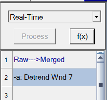
Our Real-Time flow now looks like this:

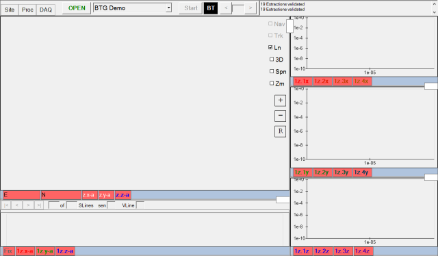
Later, when we collect data, these two functions will be run in separate threads to achieve the real-time performance. Section 5c of this manual, “Connecting Indicators”, will explain how the outputs from a flow can be connected to indicators on your display views.

Configuring your Machine’s Display Views

View Types

There are seven basic Display View Types in BTField:

Single Sensor View: Displays line plots of data collected at/or around selected positions
Gridded View: A 2D/3D gridded image of the merged EM data
Profile View: Line plots of all merged data along a sensor line
Raw Profile View: Line plots of all raw data along a sensor line
Single Response View: Bar plots of data collected at a selected position
Inversion Results View: View for navigating targets and cells, running inversions, and for analysis.
Vehicle Platform View: 3D View of the platform geometry

View Layouts

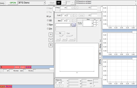
BTField supports user defined Display View layouts for each BTField project. These layouts can be further customized by the user for each machine. For example, User A may be only interested in the data collection aspect, so they may just use a layout that has as Gridded View (top left), a Profile View (bottom left), and three Single Sensor Views (right side) as shown here:

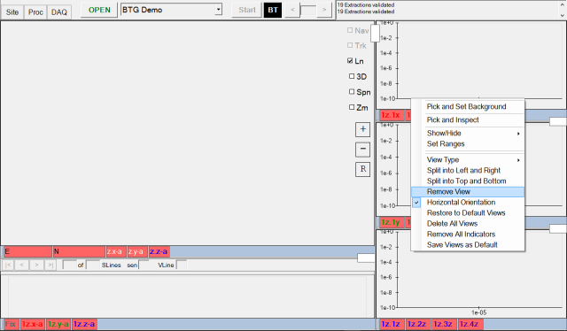
On a different machine, User B may be more interested in analyzing and inverting the data. BTField allows them to modify the layout for their machine. For example, they may not be interested in looking at the Single Sensor Views on the right side (Rx decays). They may want an Inversion Results View instead. The Single Sensor Views can be removed by right clicking and selecting Remove View like this:

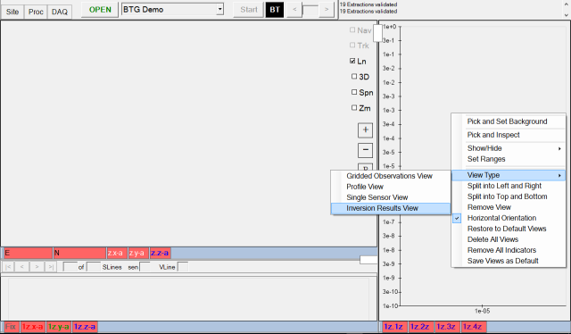
After removing the first two Single Sensor Views, the user can change the remaining one to an Inversion Results View as shown here:

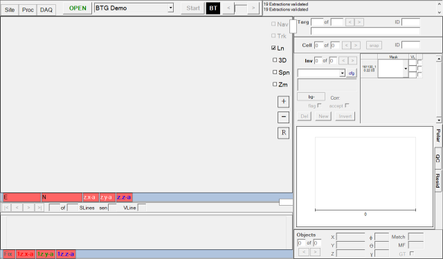
Now they have a layout that is more suited to analysis:

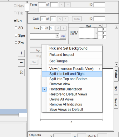
If they wanted to add the Single Sensor Views back in later, they could right click on the Inversion Results View and select Split into Left and Right:

The new panel on the right side, could then be split into Top and Bottom twice, yielding three new panels which can then be set to Single Sensor Views. Here is the final result:

Connecting Raw Data to Indicators

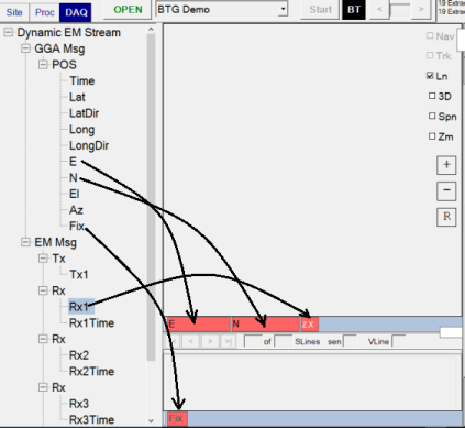
In the DAQ tab, a user can connect raw data outputs to the views using drag and drop operations as shown here:

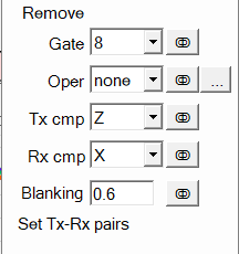
Each indicator can be configured by right clicking on the indicator. For example, an indicator on the Gridded View could be set to display the Time Gate 8 for the Z and X component combinations:

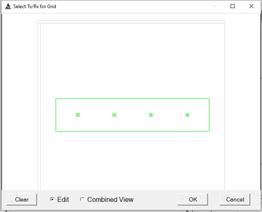
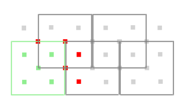
The Tx-Rx pairs also need to be set. This determines which Transmitter and Receiver pairs will be used for the gridded display when the indicator is selected. In a single transmitter system, such as what is shown below, all Tx-Rx pairs would typically be selected. Click on Edit and click on each Rx square to activate all Rx sensors as shown here:

In a multiple transmitter system, the user may only want to select specific Tx-Rx pairs to optimize the gridded display for their desired analysis. For example, in the five-transmitter system shown below, the user may only want to select Rx sensors that are close to the transmitter. The first Tx has been selected and only the 5 inner Rx sensors will be paired with it for gridding:

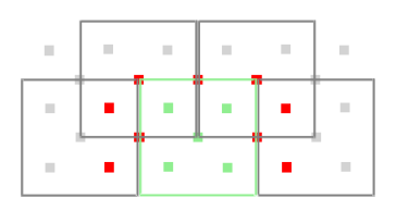
The second Tx can be selected next, and again only the 5 inner Rx sensors could be selected:

Connecting Processed Data to Indicators

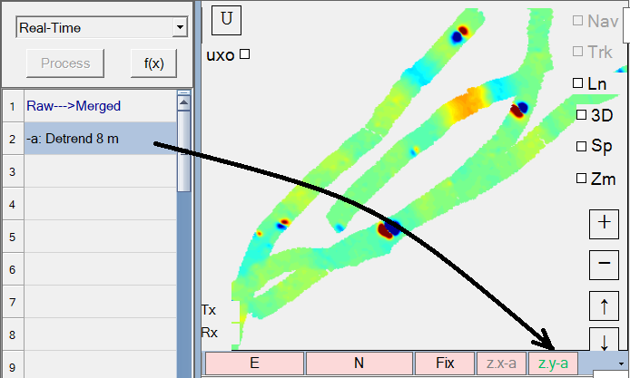
In addition to raw data, processed data from the processing flow can be connected to the indicators on a View. For example, the Detrend function at step 2 in the flow can be dragged and dropped onto the indicator bar of the gridded view as shown here:

Saving Default Views

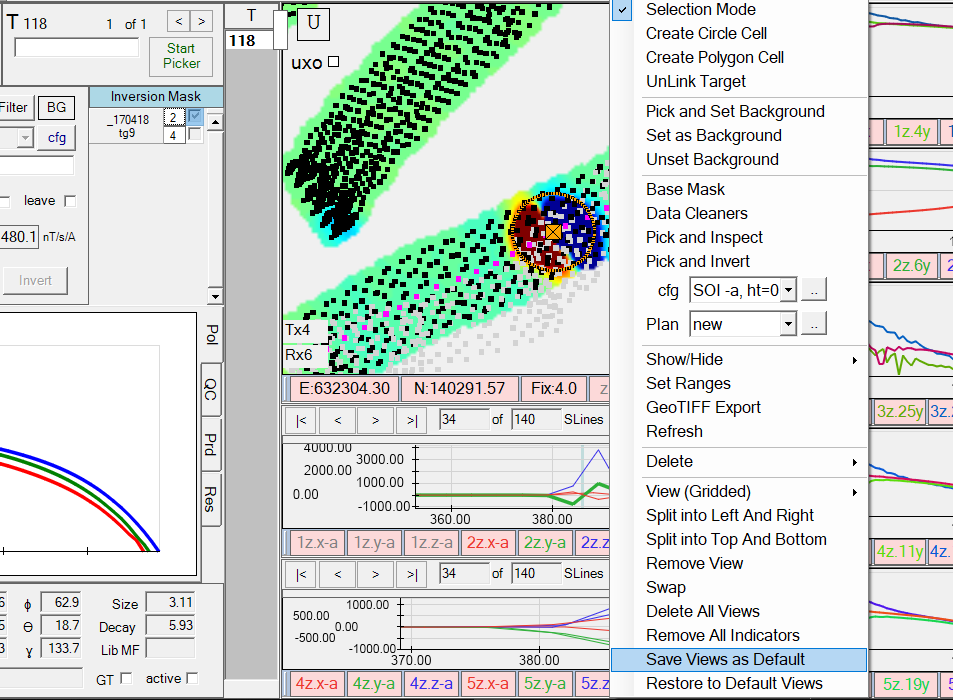
Once a user has finished configuring their views and connecting indicators for raw and/or processed data, they can save the view as the Default View of the project using the Save Views as Default function as shown here. This allows the user to use the Restore to Default Views function in the future if necessary:

Sites

Creating a Site and Survey Plan

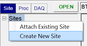
A Site is defined as a bounded area that contains multiple surveys. in the Site tab, a BTField project can attach to one or more sites using Attach Existing Site, or a new site can be created using Create New Site:

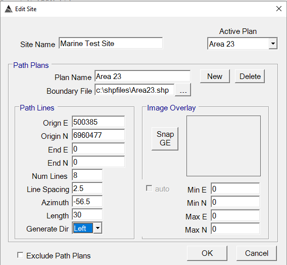
Enter the name of your site, then add a Survey Plan if desired, by clicking the New button as shown below. If you do not want to use a Survey Plan, check the Exclude Path Plans checkbox at the bottom left.

A Survey Plan will overlay path lines for the data collector operator to follow and display a boundary file for the survey using a supplied shape (*.shp) file. The straight path lines are defined by entering the appropriate values for Easting Origin, Northing Origin, Line Azimuth, Line Length, Num Lines and Line Spacing.

Registering a Google Earth Overlay

You can use the Snap GE button to automatically capture and register the currently displayed view in Google Earth. The overlay can then be selected from the Active Plan drop down list

Setting a Shape File Overlay

BTField can also overlay shape files consisting of polygons than define survey boundaries or areas to be re-collected. Set your shape file in the Boundary File field as shown above. In addition to the shp file, all other associated files such as dbf, prj, shx, qpj, must be in the same folder.

Viewing Data

Loading Surveys

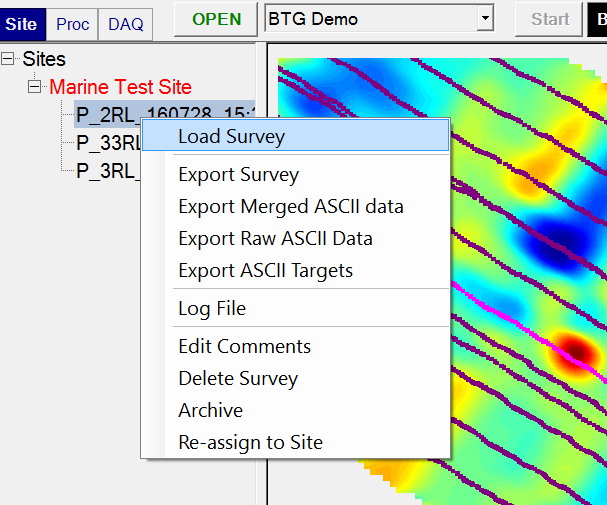
An existing Survey can be loaded by double clicking on the survey, or by right clicking and selecting Load Survey as shown here:

Gridded View

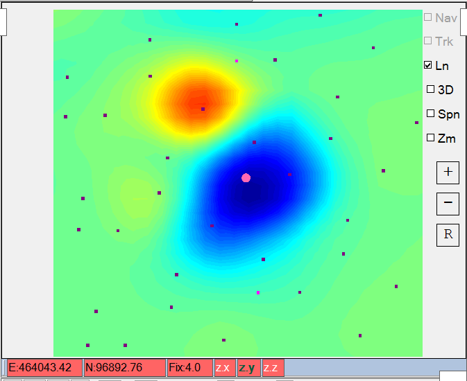
The Gridded View is the main display window that shows a gridded area of observations using the Tx-Rx-Time Gate configuration of the indicator that is currently selected. For example, the z.y indicator is selected on the Gridded View show below, displaying a grid of the observations with the z Tx loop energized and y Rx loop sensing the response:

Profile View

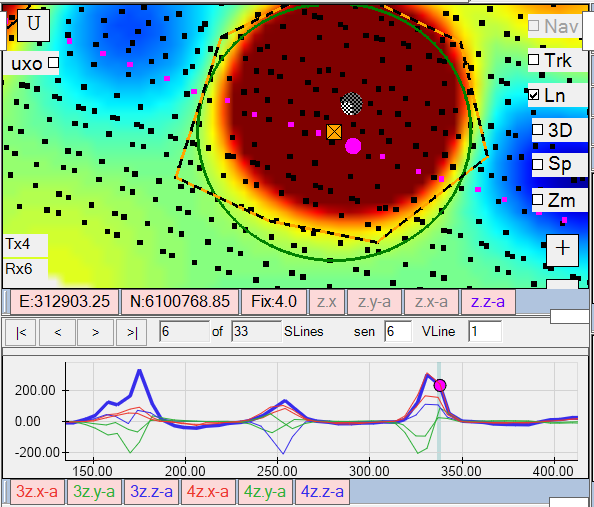
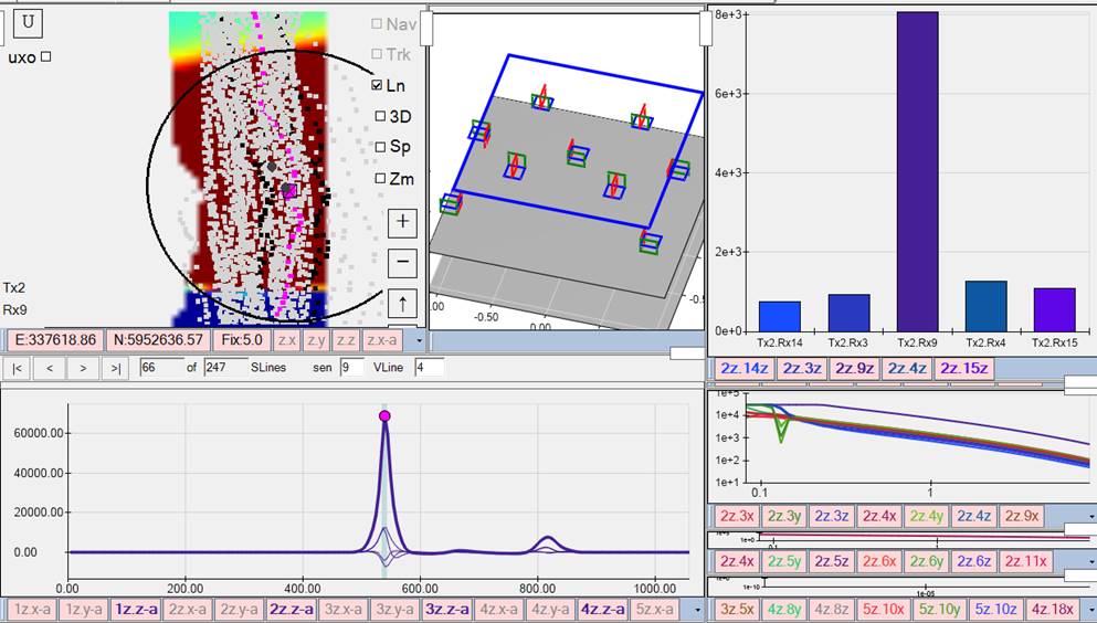
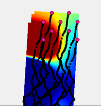
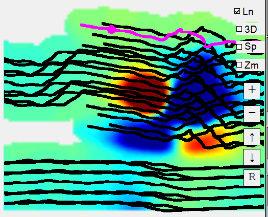
The Profile View displays all observations along a sensor line using the Tx-Rx-Time Gate configuration of the currently selected indicator. For example, the bold blue line in the Profile View shown along the bottom below, is displaying the detrended data (-a data state) for the Z loop of Rx 6 (sen 6), with the Z loop of Tx4 energizing and the Z loop of the Rx sensing the response (all noted by 4z.z -a on the profile indicator). The highlighted pink dot is the selected EM sounding location, which is also synchronized with the Gridded View above it. The blue line is in bold to indicate that its data state (-a), Tx-Rx pair combination (Tx4 and Rx6), and component combination (TxZ and RxZ), all matches the data that is currently gridded in the Grid View.

Raw Profile View

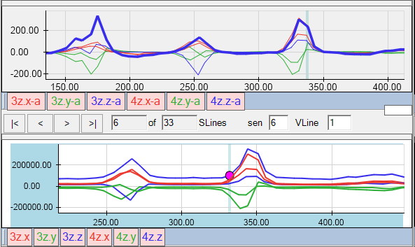
A raw profile view is sometimes required to examine data before it has been merged and normalized by the Tx current. A raw profile is shown here below the regular profile view:

Single Sensor View

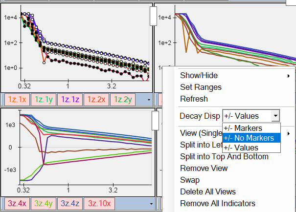
A Sensor View will display a line plot of the data values collected at a selected sounding location. The decays can be viewed with Markers (upper left), No Markers (upper right), or +/-Values (bottom left):

Inversion Results View

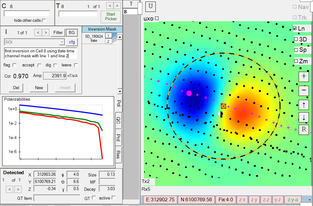
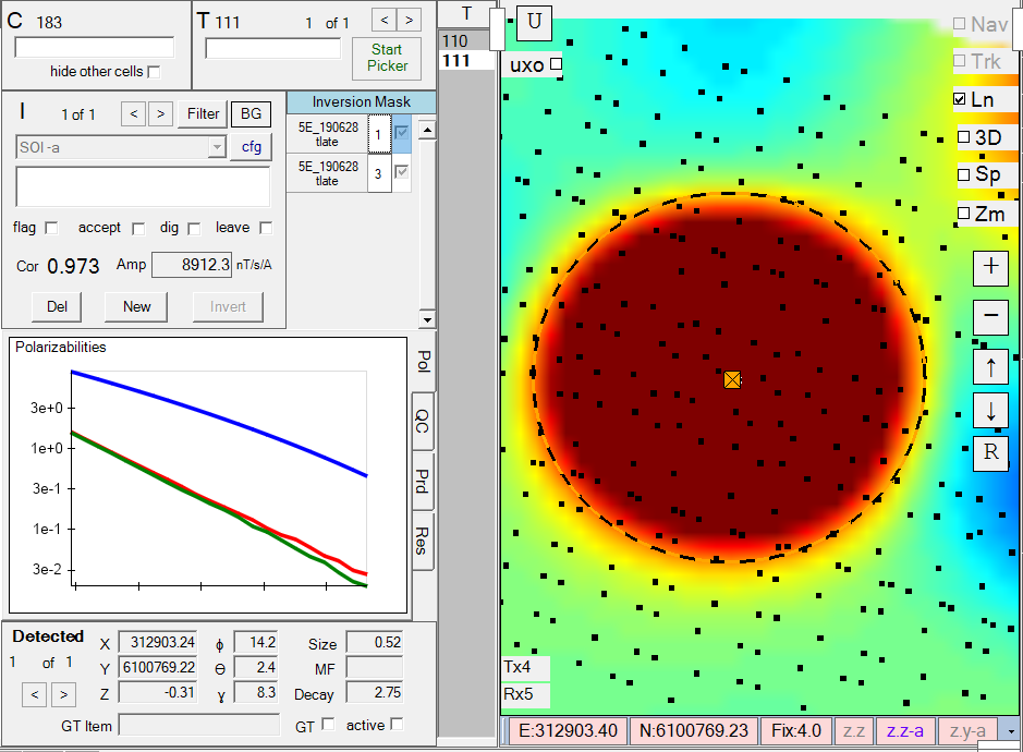
The Inversion Results View is the main view for navigating targets and cells, running inversions, and analyzing classification results. The example below shows the inversion results for a circular cell created around a target pick (orange square). The resultant polarizabilities are shown on the left with and correlation of 0.970

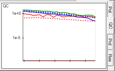
The QC tab will display observed and predicted data for a selected sounding location within the cell, using solid and dashed lines respectively:

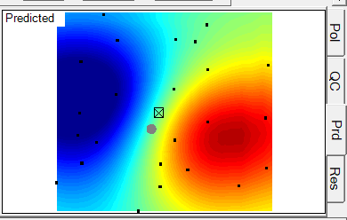
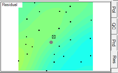
The Pred and Resid tabs, will display a gridded view of all sounding locations within the circular cell, allowing the user to immediately compare them with observed cell selected in the Grid View

Single Response View

The Single Response View can be used for displaying responses from specific Tx-Rx pairings on bar graphs. This can provide an easy way to determine the approximate xy location of an anomaly during data collection. For example, here is a marine system using the full mode with a Single Response view set up for the inner sensors. As the platform passes over the anomaly the bars indicate the Z component response:

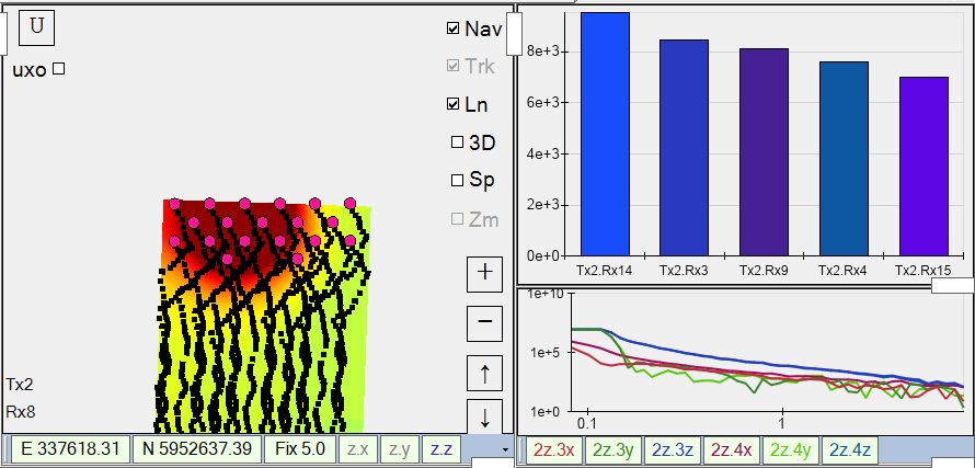
Here is another example with the platform running in the eod2 mode with only the inner sensor active. In this case the platform is passing directly over an anomaly, yielding a dominant response on the middle Rx9 sensor:

Vehicle Platform View

The Vehicle Platform view provides a 3D zoom/rotatable model of the system. The platform height can be adjusted up or down, and the visibility of each Tx/Rx sensor can be toggled to fully verify sensor geometry.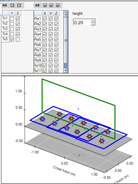

Data Collection on the Control Computer

Project Settings for Data Collection

To edit the project settings for data collection, click on the black square BT button at the top of the application:

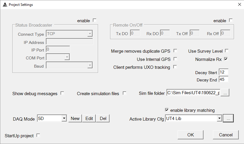
Open the Project Settings window and configure the settings for your project. Here is a description of each option:

Status Broadcaster: sends status messages to an external system to indicate data quality.
Night Mode: uses a black background with high contrast text and plots.
Using Internal GPS: option for testing without valid GPS data.
Using Survey Level: option to require a Survey Level selection when opening a new survey .
StartUp Project: determines if the current project will load first when launching BTField.
Normalize Rx: when checked, the merged EM observations will be normalized by the Tx current.
Show debug messages: determines if extra diagnostic messages appear in the status window.
Create simulation files: determines if the raw sensor stream data will be saved to disk for the purpose of analysis, or to add a new simulation stream to the BTG Server.
DAQ Mode: a selectable mode of operation for data collection. Each mode can use different data consumption settings and include/exclude different sensors.
Active Library Cfg: selects the munitions library that will be used for determining the best library item match after performing an inversion.

Connecting to Sensors

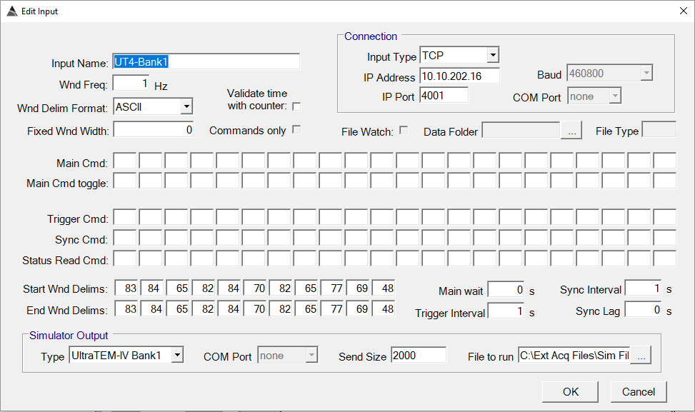
In the field, a data collection computer is always the Control Computer because it hosts the database and it allows the operator to Start and Stop data collection. The Control Computer will be connected to the sensor inputs using the Input settings in the DAQ tab. Right clicking on an input node will allow you to Edit the input settings as shown below. This example shows a connection to a TCP stream of EM data found at IP 10.10.2002:16 on port 4001. Alternatively, BTField can connect to serial COM streams for sensors that do not output TCP or cannot be connected through a Serial Device Server (a device that converts serial COM to TCP).

Survey Types

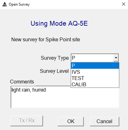
Before opening a new survey, the real-time processing flow should be configured as described in section 4 – Configuring the Real-Time Flow. Once the real-time flow is configured, click the OPEN button to open a new survey. Type in any relevant comments, and select either a P (production), IVS, TEST, or CALIB (calibration) survey type:

P: Production {#ProductionSurveys} Surveys: All dig/no dig decisions are made from the inversion results of P surveys. A P survey can only be collected using a BTField project that is registered by Black Tusk Geophysics. Also note that the Master survey for a site can consist only of P Surveys.
IVS: Instrument {#IVSSurveys} Verification Strip Surveys
TEST: Test Surveys: {#TestSurveys} A TEST survey is typically used during project development, before the project is registered by Black Tusk Geophysics.
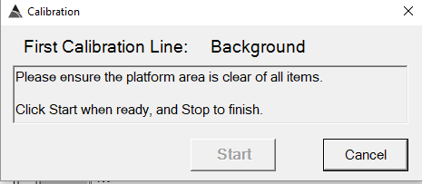
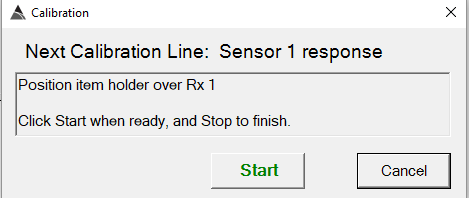
CALIB: {#CalibrationSurveys} Sensor Calibration Surveys. When opened, the CALIB survey will instruct the user to first collect a background measurement, then ask them to move the test item from sensor to sensor while collecting data using the Start/Stop line button as shown here:

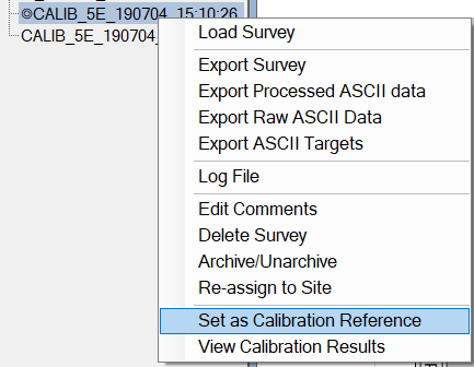
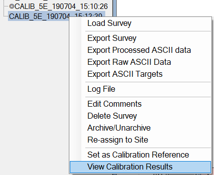
Any CALIB survey can be set as the Calibration Reference as shown on the left. Once the calibration reference survey is set, other CALIB surveys can be compared to it by selecting View Calibration Results as shown on the right:

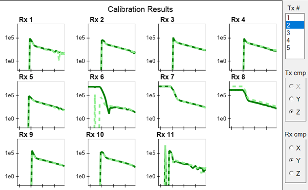
Here is an example of the sensor calibration results for a 5 Tx, 11 Rx system. Any combination of Tx and Rx components can be viewed. The calibration reference responses are shown with a dashed line, while the responses being tested are shown with a solid line:

Navigation modes

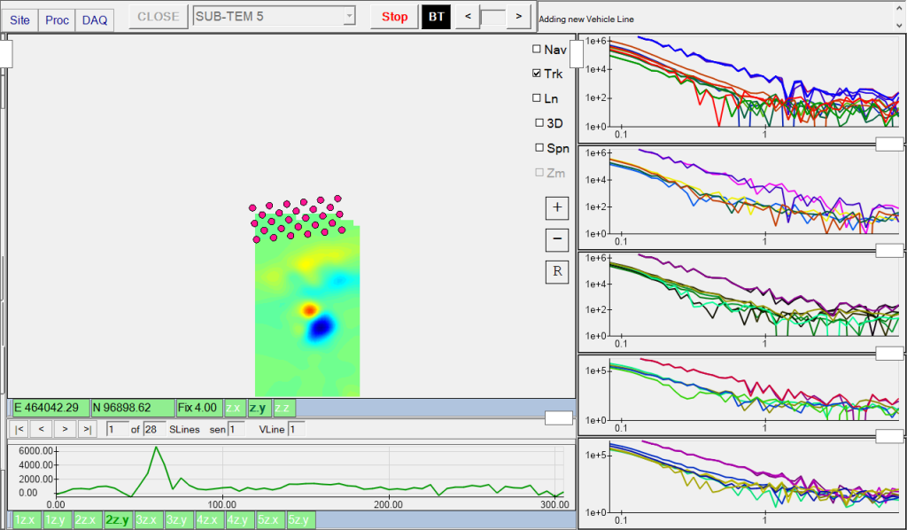
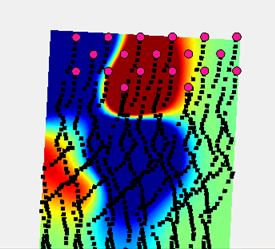
Once data is streaming, click the Start button to begin data collection along the first vehicle line. The real-time grid will appear as shown below, indicating that data is being collected and saved to disk. The small round, red circles indicate the sensor positions on the platform. At any time, the user can switch between a vehicle-centric view and geographic view using the Nav checkbox on the top right side of the Gridded View. The user can also use the Trk button to switch between tracking mode and analysis mode if they wish to inspect or invert an area while the data collection is still active.

Coverage History

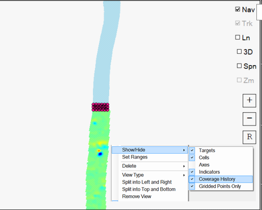
During data collection, the user can display a light blue path for all surveys previously collected in the Site. Right click on the Gridded View and select Coverage History as shown here:

Real-Time Classification

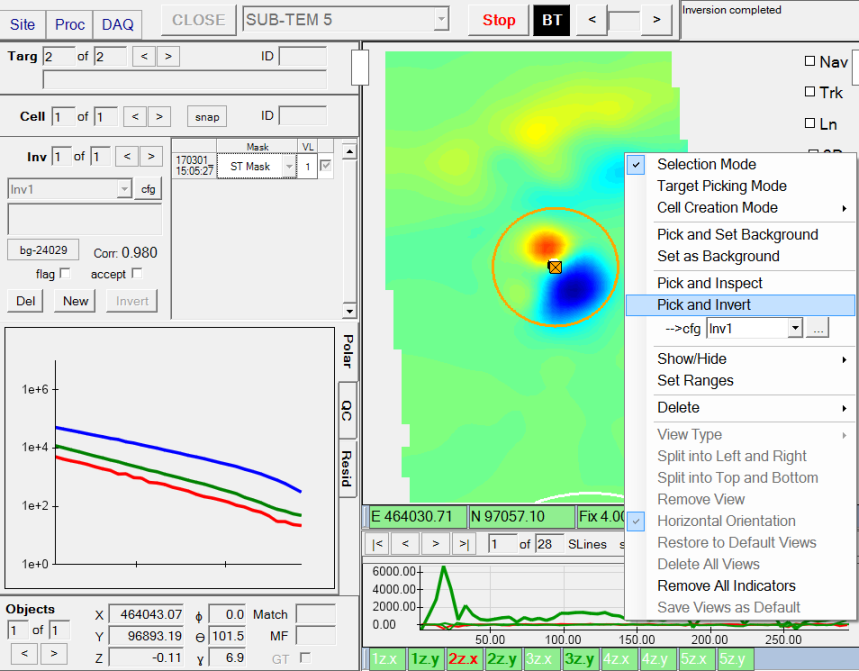
During data collection, the user can exit tracking mode by unchecking the Trk checkbox, allowing them to zoom in on an anomaly of interest and immediately invert it using the Pick and Invert tool as shown below. The Pick and Invert tool allows the user to click and drag outward to create a target and cell, followed by a mouse release that immediately runs the inversion. This provides an easy method of quickly investigating an anomaly in real-time without stopping data collection.

Real-Time UXO Tracking

BTField can also perform real-time uxo tracking if the user creates an inversion configuration with the “UXO tracking” option checked. This provides a robust way of tracking uxo in real-time since full inversions are continually being performed on the incoming data. An example of an inversion configuration with uxo tracking enabled is shown below:

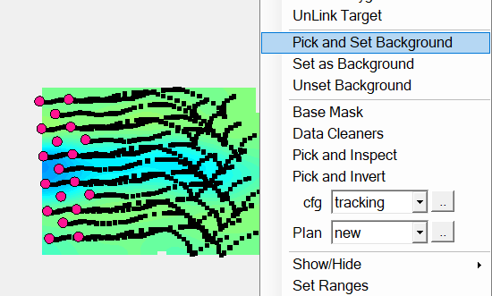
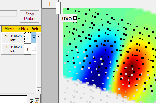
Note that the inversion configuration we are using for uxo tracking in this example is using the unfiltered (unfilt) data as input, allowing the inversion to proceed as soon as the data arrives. Therefore, a background needs to be selected first. Once a new line is started, use the Pick and Set Background tool to set the background:

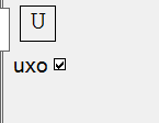
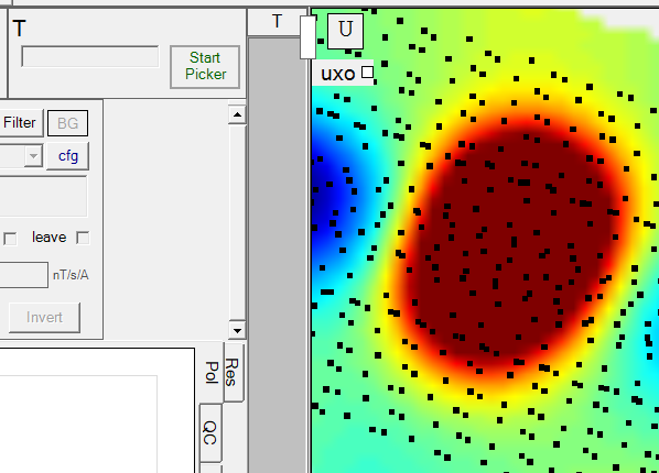
Now the “uxo” checkbox can be switched on in the upper left corner of the Grid View:

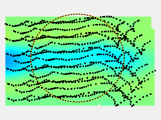
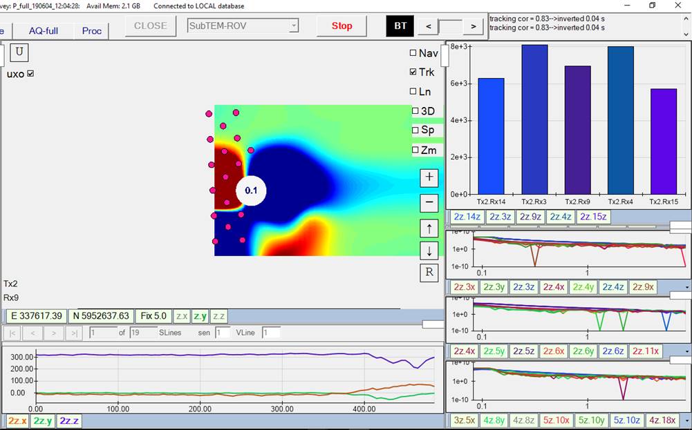
Here is an example of the uxo tracking switched on as it continually inverts the most recently consumed data: The white circle in the screenshot below indicates an item detected at 0.1 m above the ground (in this case, a test item resting on the ground surface). In the upper right corner, you can see that BTField is inverting the current location with a 0.83 correlation (recall the threshold for showing the white dot was set at 0.78 in the inversion configuration). The white dot will keep displaying over the detected location as long as the platform is near the item. Once the platform moves completely past the item, the track will be dropped.

Switching between DAQ Modes

Some sensor platforms have the ability to operate at different frequencies, and/or have different sensors active, and/or can be configured with different sensor geometries. BTField allows the user to easily switch between these different modes of operation using the DAQ Mode drop down list in the Project Settings dialog. This allows all users to remain within the same BTField project while continuing to collect, analyze, and process data regardless of the mode. It also allows the creation of a Master survey that can contain a mix of surveys collected in these different modes.

Here is a sample marine project where three modes have been created. They are named full, eod1, and eod2, and they are selectable from the Project Settings:

In the DAQ tab, each mode looks very similar, except that some sensors may have different data consumption settings, and other sensors may be excluded. In the “full” mode show below, transmitter 6 (Tx6) is excluded while the other five Tx and all eleven Rx and included:

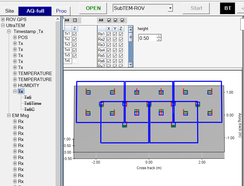
During collection, the operator will see all eleven Rx consuming data:

If the operator switches to the “eod2” mode, for example, then only Tx2 (the front-middle rectangular loop) and Tx6 (back-middle figure 8 loop) are actively transmitting, with only the middle nine Rx sensors (3, 4, 8, 9, 10, 14, 15, 18, 19) actively sensing:

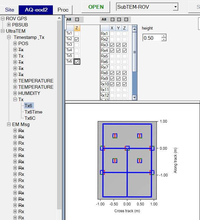
Now during collection, the operator will see only the middle nine Rx consuming data:

BTField will allow a Master survey to be created using surveys collected in each of these modes. Here is a Master survey example that combines our full and eod2 surveys:

The Master survey provides additional control to turn off specific vehicle lines. For example, if the user wanted to look at only the full mode data in this area, they can turn off lines 2 and 3 which were collected with eod2:

Real-Time Classification from a Networked Client Computer

For data collection, there is an option to add another BTField computer that will connect to the database running on the Control Computer (the data collection computer). This new client machine will then be able to Join an active survey and display the real-time grid. At any time, the user on the client machine can switch the tracking (Trk) off to perform real-time inversions using the Pick and Invert Tool. This allows the data collection operator to focus only on data collection, while the leaving the real-time analysis to another user on the client machine.

To accomplish this, the two machines must be networked either wired or wirelessly. When launching BTField, the client machine must connect to the Control Computer’s IP address and computer name. Below is an example of a client machine connecting to the Control Computer named COLLECTOR_1 that has a LAN IP address of 192.168.1.3

Post-Processing

Configuring Post-Processing Flows

Once data has been collected, it has been processed by the Real-Time flow. All Real-Time flows have a Merge function labelled RawMerged, therefore, at a minimum, the collected data will be merged to the time base of the EM sensors. If the Detrend function was also included in the real-time flow, the data would be considered “processed” and immediately ready for inclusion in a Master survey where target picking and inversions are typically performed. However, if the Detrend function was not used in the real-time flow, a post-processing flow would be required to detrend the data.

There are six post-processing flows available:

S1 for Single: used for auto-processing single surveys on import, and for batch processing.
S2 for Single: An additional flow for processing single surveys.
S3 for Single: An additional flow for processing single surveys.
M1 for Master: used for auto-inverting master surveys after target picking.
M2 for Master: An additional flow for processing master surveys.
M3 for Master: An additional flow for processing master surveys.

For example, we can configure the S1 for Single flow by clicking the f(x) button and dragging in the Detrend function to prepare the data for inversions:

Now any single survey can be loaded and detrended by clicking the Process button.

Batch Processing Surveys

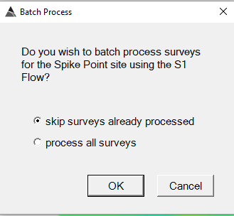
All Production surveys can be processed at once by the S1 for Single flow by right clicking on the Site and selecting “Batch Process Surveys”. The user has the option of processing or (re-processing) all surveys, or skipping surveys already processed:

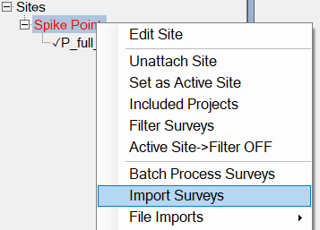
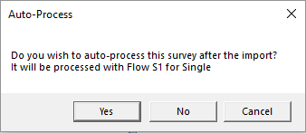
The user also has the option to run the S1 for Single flow during import of a survey(s):

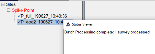
After the survey(s) have been processed, a check mark will appear in front of the survey name to indicate it is ready for inclusion in a Master Survey:

Creating a Master Survey

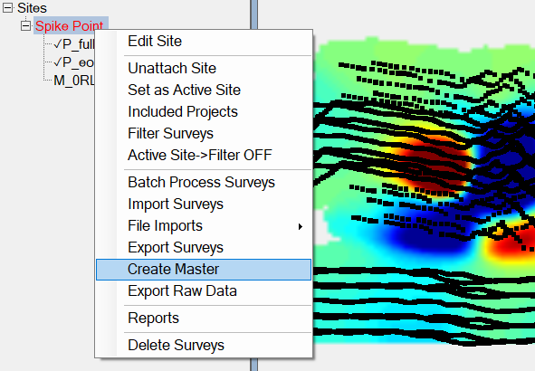
To pick targets and invert data collected across multiple surveys within a site, a user can create a Master survey for the site. Right click on the site’s name and select Create Master as shown. The Master survey will load and display all processed (detrended) surveys for the site

As new surveys are added to the site, the Master survey will automatically update itself. Target picking and inversion can now be performed while having access to all historical data collected over each anomaly.

Picking Targets

Targets can be picked in either a Single Survey or in the Master Survey. It is recommended to pick targets in the Master Survey since it allows the user to visualize all historical data collected over the anomaly. To pick targets, an Inversion Results View must be added (see Section 5 – Configuring Your Machine’s Display Views). With the Master Survey loaded, click on the Start Picker button in the Inversion Results View:

Once the Picker is started, it will display the single surveys and line numbers found within the currently zoomed area. Pressing the X key while left-clicking will pick the target:

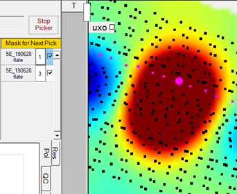
If desired, specific lines can be unchecked to achieve the optimal visualization of the data to be inverted. For example, line 3 can be unchecked to visualize the gridded Y component:

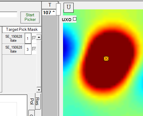
Once the target is picked, it will retain the visualization that was used for the pick decision. The Picker can be started again at any time to continue picking more targets:

Inverting Data

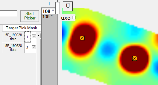
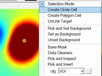
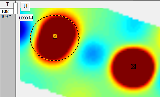
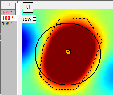
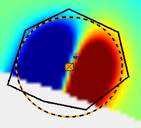
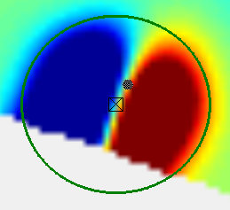
To invert data around a target pick, a cell must be created first. Cells can be circular, or polygon shaped. For example, a circular cell can be created around the target 108 by right clicking and choosing “Create Circle Cell” from the menu. Click, hold, and drag out to display the circular cell, then release to create it:

Note that target 108 now has its hat (^) symbol removed in the target list, indicating that it is now associated with a cell:

To create a polygon cell, select “Create Polygon Cell” from the menu, click successive points, then press Enter to close the polygon. Note that in our example, target 108 now has two cells associated with it. The red color in the target list indicates that a decision will be required to select the cell with the best inversion results:

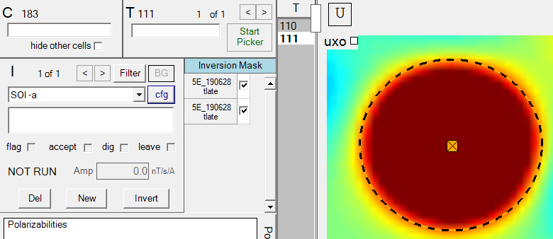
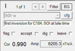
Once the cell is created, the user can invert the data within it by clicking the Invert button. The inversion will proceed using the currently selected Inversion configuration. For example, in the screenshot below, the “SOI -a” inversion configuration will be used when the user clicks the Invert button (SOI stands for Single Object Inversion). The settings of the inversion configuration can be accessed using the blue “cfg” button.

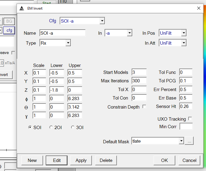
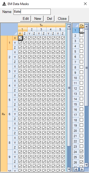
If we click on the cfg button, we can inspect the SOI -a inversion configuration as shown below. It accepts the detrended -a data state as the In parameter, while using the unfiltered data states of position (In Pos) and attitude (In Att). The horizontal bounds are set to constrain the xy fit location to within +/- 0.5 m from the target pick location. The vertical fit location is constrained to be between ground level and -1.8 m. The sensor height is set to 0.26 m, which was the platform height above ground during collection. The Default Mask is tlate, which has only the late time channels selected (gates 24 to 45). When a new cell is created, the data masks for all lines falling within the cell will default to use tlate.

Once an inversion configuration is created, any cell can be inverted by clicking the New button to create a blank inversion for cell. The Invert button can then be clicked to invert the cell data. The inversion results will be immediately displayed as shown here on the left side:

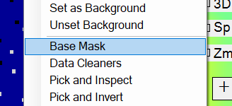
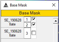
The user also has the option to pick a target, create a cell, and perform the inversion in one step using the Pick and Invert tool. In the example below, the user has decided to first mask out an unwanted line using the Base Mask, which is available off the right click on the Grid View as shown here:

Next, they select the Pick and Invert tool from the menu and click, hold, drag out and release to perform all three operations at once:

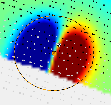
As soon as the user releases the mouse button, the data within the cell will be inverted. The detected location will show on the grid as a black and white checkered ball. Here are the results, showing a 9.90 correlation fit to the dipole model and the three principal axis polarizabilities of the item:

Batch Inverting Surveys

A user may want to pick several targets first before inverting data. In this case it can be helpful to use the M1 for Master flow to automatically create circular cells around each target and auto-invert the data. For example, on the right is the M1 for Master flow set with Auto-create Cells using a radius of 0.5 meters, followed by an inversion that uses the EM Invert SOI inversion configuration.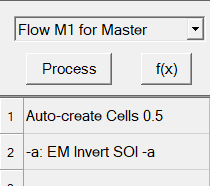

The user can run the flow at any time to invert recently picked targets. Therefore, a user can pick some targets, run the flow to batch invert and inspect results, then pick more targets, etc.

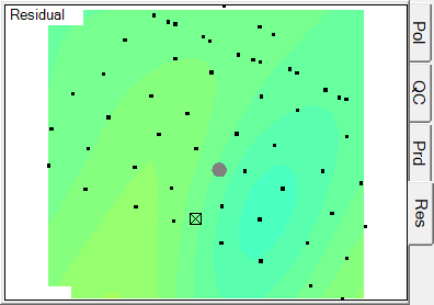
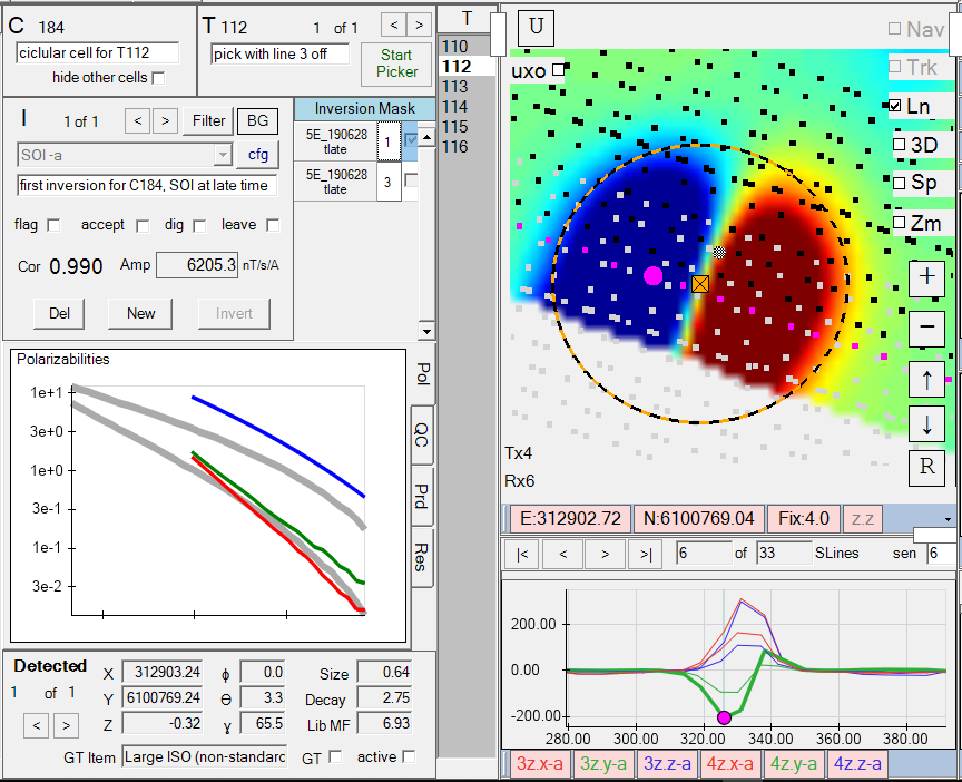
g. Analyzing Inversion Results

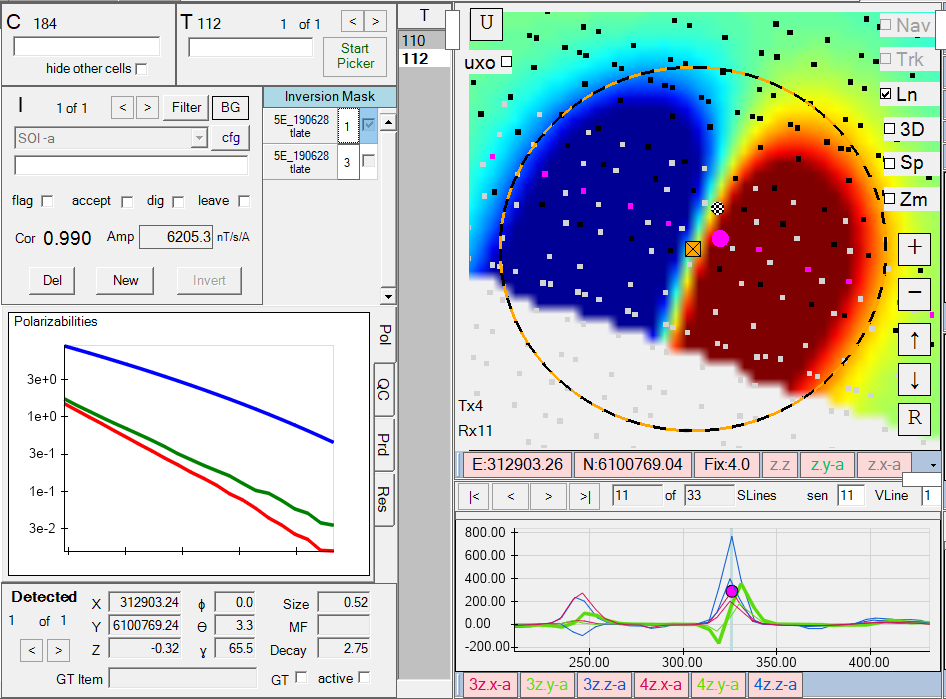
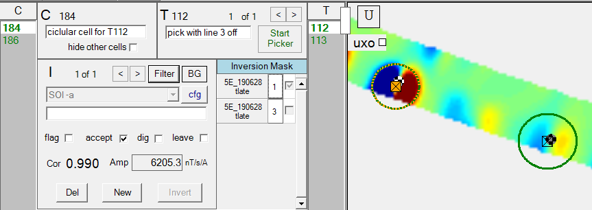
The Inversion Results view displays all calculated values from the inversion operation, including gridded views of the predicted and residual that provides immediate comparison to the observed data on the Grid View. For example, in the right screenshot Cell 184 was inverted using the SOI -a inversion configuration which uses the late time channels as specified in the tlate mask. This inversion was performed with line 3 turned off, and it is the first inversion for Cell 184. The inversion is showing a high 9.90 correlation (Cor) fit to the dipole model. In the Pol tab, the principal axis polarizability (blue) response is higher than the two similar transverse principal axis polarizabilities (red and green). This indicates the item has one long dimension and is symmetric about the other two dimensions (i.e. consistent with a uxo shape or metal rod).

The amplitude (Amp) is a summation of the inverted EM observations. The value of 6205.5 nT/s/A is taken from the Tx/Rx pair having the maximum summation. Note that the Amp measure is dependent on the inverted time channels, therefore cells must be inverted with the same inversion mask to allow accurate comparison of Amp between items.

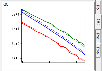
The QC tab (left image below) provides a visual comparison between observed (solid lines) and fitted (dashed lines) data. Any location within the cell can be selected to display these plots for a specific Tx/Rx pair.

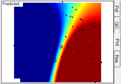
The Pred tab (middle image below) displays a gridded view of the predicted data, using the visualization settings of the currently selected Grid View indicator. This allows for easy comparison to the observed data in the Grid View.

The Resid tab (right image below) displays a gridded view of the residual data. Our example reveals very little residual, as would be expected with a high correlation 9.90 fit.

The Detected Panel at the bottom of the Inversion Results view displays the best XYZ fit location of the item in meters. The X and Y values are represented in Easting and Northing, while the Z value is the depth below the surface. The best fit orientation of the item is shown using the angles of azimuth φ , dip ϴ, and rotation ɣ. In our example below, azimuth = 0.0 degrees and dip = 3.3 degrees, indicating the long axis of the item is almost vertical and aligned to UTM north. The rotation about the long axis is 65.5 degrees.

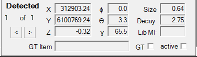
If the Correlation fit is sufficiently high (above 0.80 ), the Size can also be valuable for determining the presence of uxo. If only larger items are of interest, the Size measure can be used as a threshold. Note that the Size measure is dependent on the inverted time channels, therefore cells must be inverted with the same inversion mask to allow accurate comparison of Size between items.

If the Correlation fit is sufficiently high (above 0.80 ), the Decay can also be valuable for determining the presence of uxo. most uxo will have slow decaying polarizabilities that extend into late time before dropping off to near zero. Some users will see this immediately by examining the polarizability curves, but it will also be quantified by the Decay measure, which will typically be lower for uxo items.

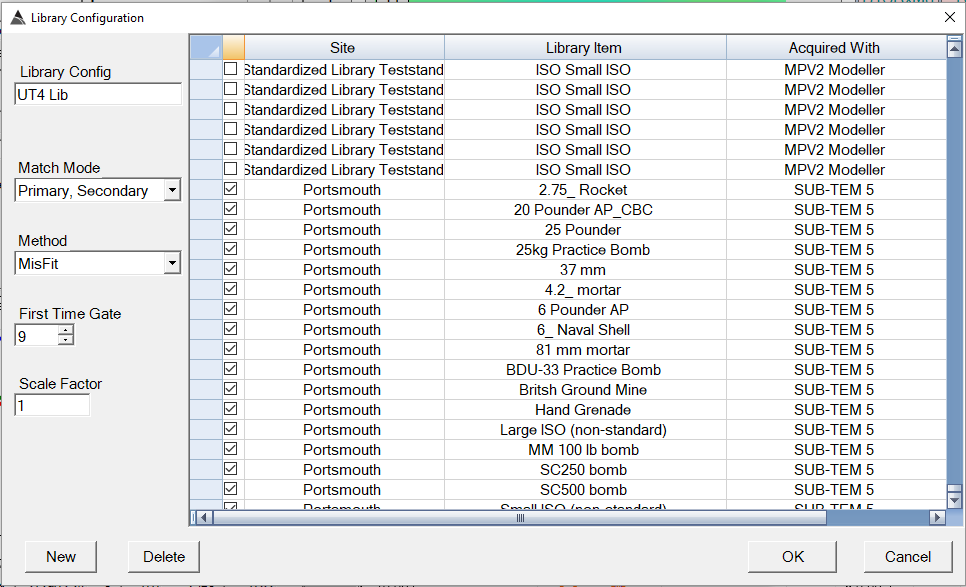
Creating and Using a Munitions Library

In the Inversion Results window, any inverted item can be marked as a ground truth (GT) item. This will make it immediately available for inclusion in a munitions library. In the Project Settings window, a munitions library can be created by selecting any number of ground truth items that may be present at the survey site. Below is an example of a library named UT4 Lib that was configured by selecting GT items collected at the Portsmouth site. The Match Mode can be set to match all polarizabilities, or just primary and secondary, or primary only. In our example here we have chosen to match the primary and secondary polarizabilities. The selected GT items were all inverted using time channels 9 to 45, therefore the First Time Gate must be set to 9.

After setting the library configuration, we can enable it as shown here in Project Settings:

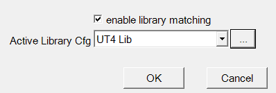
Now the all inversions for this BTField project will display the best match to the items in the active library. Below, our inverted example is indicating the best match is a Large ISO item with a library misfit (Lib MF) of 6.93. The library polarizabilities are plotted in grey for visual comparison to the inverted polarizabilities. Recall that our library configuration has its Match Mode set to “Primary, Secondary”, therefore only 2 grey lines are displayed. Also recall that the First Time Gate of all the selected library items is 9, but we are only inverting the late time gates (24 – 45). The plot automatically aligns the polarizabilities to their proper time ranges.

Setting QC Status and Filtering Inversion Results

In the Inversion Results view, there are four QC status states: flag, accept, dig, and leave.

A flag checkmark indicates a potential uxo item. This means the current inversion results are good enough warrant further investigation/analysis.

An accept checkmark indicates a detected uxo item. The inversion analysis of the anomaly has been concluded and the inversion results support a decision to classify the anomaly as a uxo. When a user checks accept, all other cells and inversions associated with the target will automatically hide, and the accepted cell with turn green as shown here:

The dig check indicates the item should be excavated and removed.

The leave check indicates that although item has been flagged or accepted, a decision has been made to leave the item in place. This decision is sometimes made when excavation and/or removal of the item is unsafe, and leaving it in place is the safer option.

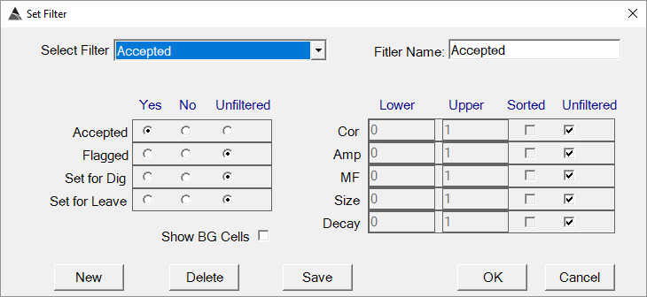
Filters can also be applied to sort on QC status and inversion results. Click the Filter button in the Inversion Results window to select or create a filter. For example, the “Accepted” filter is selected below:

After clicking OK, the Cell and Target lists, and Grid View, will show only accepted cells and inversions

Generating Reports

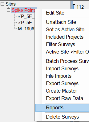
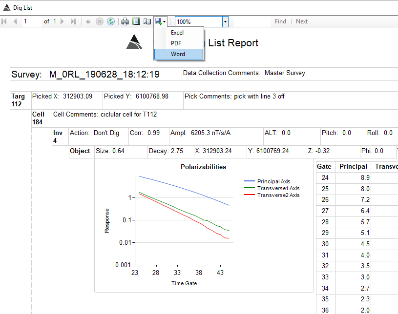
To generate a report, a Master survey must have been created for the site. Right click on the site and select Reports:

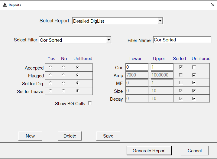
The Reports dialog will show, allowing you to select a report and optionally apply filters. For example, the Detailed DigList report can be selected and generated using a filter that will sort the items in descending order of correlation:

The report will be generated on screen, and it can then be exported to Excel, PDF, or Word using the drop down list shown here at the top of the report:

Transferring Data between Networks

Exporting Surveys

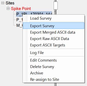
If two BTField machines are on the same network, there is no need to export or import surveys. All BTField machines on the network can connect to the Control Computer that is hosting the central database. However, if a non-networked machine has data that needs to be transferred, the survey(s) can be exported using the Export Surveys feature. To export an individual survey, right click on the survey and select Export Survey as shown:

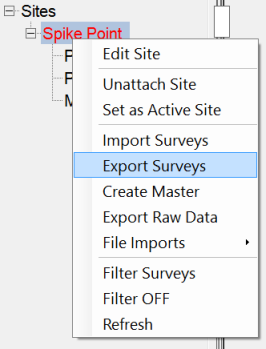
To export all surveys for a site, right click on the Site and select Export Surveys as shown:

An export folder containing the data will be created on disk. The folder name will contain the site name, the number of surveys exported, a “SurvExp” label, and a timestamp. For example, the export shown above created an export folder named “Spike Point(1 survey) SurvExp -2017-03-01 at 18h11m37s”

Importing Surveys

Surveys can be imported using the same right click menu as shown above, and selecting Import Surveys to point BTField towards a folder with a matching site name.

Exporting Processed ASCII data

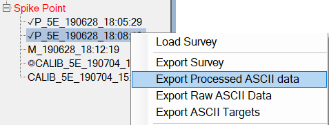
If the merged data needs to be exported to an external system (i.e. an application other than BTField), an ASCII export will be required. Right click on a survey and select Export Processed ASCII data.

Exporting RAW ASCII data

If the raw data needs to be exported to an external system (i.e. an application other than BTField), an ASCII export will be required. Right click on a survey and select Export Raw ASCII data. The folder name containing all raw data files will have the RawExp label, Site name and date. For example, “RawExp-Spike Point, P_1RL_170301_14-06-28”

Exporting a GeoTIFF

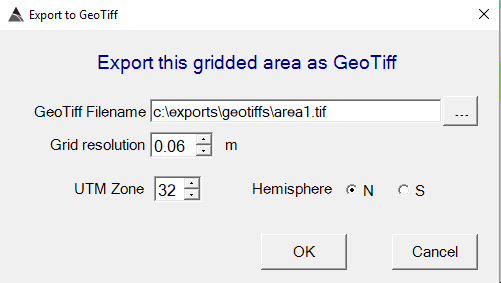
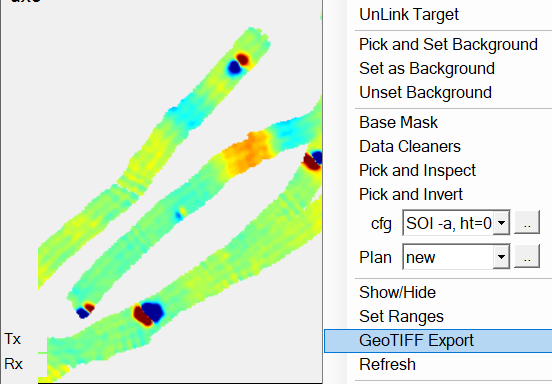
The currently zoomed area displaying on the Grid view can be exported as a GeoTIFF by right clicking and selecting GeoTIFF Export as shown:

If the survey was collected with BTField v12.14.0 or higher, the UTM Zone and Hemisphere will auto-fill. Set the Grid resolution to meet your requirements:

Tags: