Overview
BTField applies a polarizability post-processing step that conditions inverted polarizability curves before they are used for library matching. The pipeline is a faithful port of the UXOLab QCZilla logic and runs in a fixed order:
- Zero / negative interpolation (always) — for each axis, any gate with a value ≤ 0 is replaced by the mean of its two nearest gates that are > 0. If an axis has no positive gates it is filled with a tiny constant.
- Initial whole-curve relabel (always) — the three axes are ranked and relabelled so the axis with the largest summed response becomes L1, then L2, then L3. The whole axis array moves as a unit; only the ranking metric is a sum. BTField computes that ranking sum over only the late-time gates (time > 0.262 ms). (If no gate exceeds the threshold, it falls back to summing over all gates.)
- Population de-spike (optional) — a per-gate, per-axis spike threshold is built from the whole survey population (median of
log10(L) - threshold); values below it are treated as spikes and replaced by the mean of the two nearest non-spike gates. - Floor (optional) — values below the floor are clamped up to the floor.
- Final sort — a final ordering pass whose mode is user-selectable:
- Whole-curve sort (default) — the same time-gated, sum-based relabel as step 2 (each axis array kept as a unit).
- Per-gate sort — the three axis values are sorted independently at each time gate so that L1 ≥ L2 ≥ L3 at every gate.
Both the raw and the processed polarizabilities are kept:
- The raw curve is stored in a
.polrawrecord and is never overwritten by processing. - The processed curve is stored in a
.polrecord and is what library matching uses.
Processing runs automatically on inversion, HDF5 import, and library import, and can also be run on demand (see below). Processing settings are stored per DAQ configuration (for predicted/survey pols) and per library survey (for library pols), so they travel with the data.
Processing settings
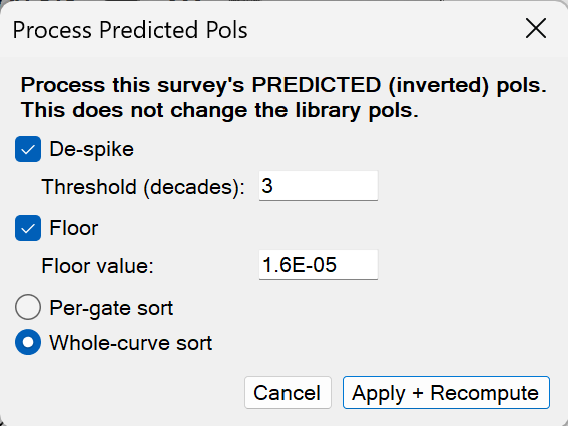
The processing settings dialog exposes the de-spike, floor, and sort options described above.
| Setting | Purpose |
|---|---|
| De-spike | Enables population-based removal of isolated spikes. |
| Floor | Minimum value applied to the curve after de-spiking. |
| Sort mode | Controls the whole-curve and final sort behaviour. |
Process Predicted Pols (per survey)
Use Process Predicted Pols to (re)process the polarizabilities of the currently loaded survey — for example after changing a processing setting, or to apply processing to legacy inversions.
The dialog is launched from the small bold P button on the Inversion Results panel (next to the library controls). Hovering the button shows the tooltip “Process this survey’s PREDICTED (inverted) pols (de-spike / floor / sort), then recompute matches. Does not change the library pols.”
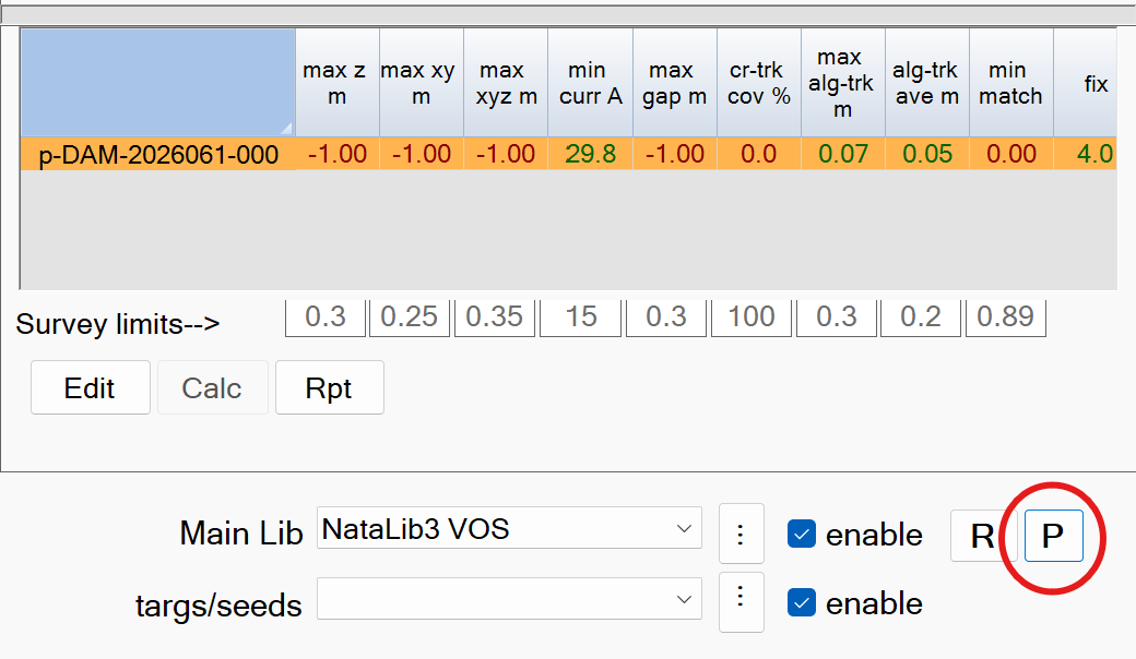
Clicking P opens the settings dialog. Choose the de-spike, floor, and sort options and click Apply + Recompute to reprocess the survey’s predicted pols from the raw pols and recompute matches.
Process Library Pols (shared library)
Use Process Library Pols to process the polarizabilities of a shared ordnance library. The library’s processing settings are stored with the library survey so all users matching against it get consistent processed curves.
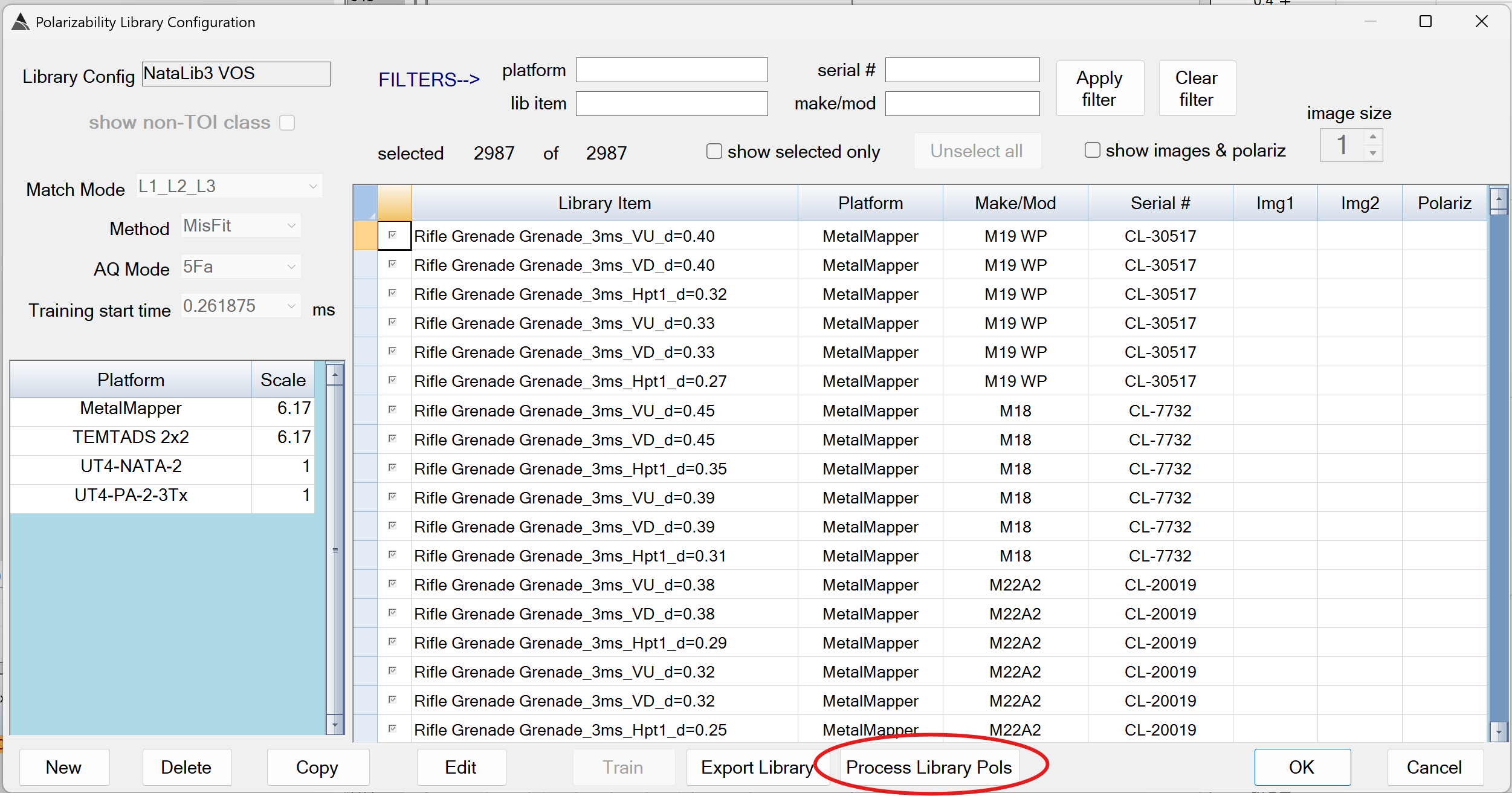
The Process Library Pols button is on the bottom panel of the Library Configuration form. Its tooltip reads “Reprocess and overwrite the shared library pols for ALL projects from the raw pols (de-spike / floor / sort). The raw pols are not changed.”
Adding Pol Process to the Auto-invert flow
Instead of processing pols on demand, you can add a Pol Process step to the Auto-invert flow so that every inversion is pol-processed automatically. The step runs after EM Invert and applies a named processing configuration.
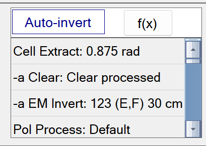
To add the step, open the Auto-invert flow editor (the f(x) button) and insert a Pol Process function after EM Invert. Configure the step by selecting or creating a processing configuration:
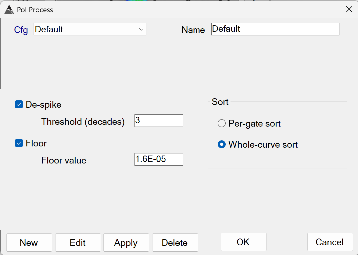
- Cfg / Name — select an existing named configuration (for example Default) or create a new one. The selected config’s de-spike, floor, and sort settings are applied every time the flow runs.
- New / Edit / Delete — manage the saved configurations.
- Apply — save changes to the selected configuration.
- OK — accept the configuration for the flow step.
Once the Pol Process step is part of the flow, running Auto-invert produces processed pols (used for matching) automatically, with no separate manual step. The de-spike, floor, and sort options are the same as described in Processing settings.
Raw vs. processed curves
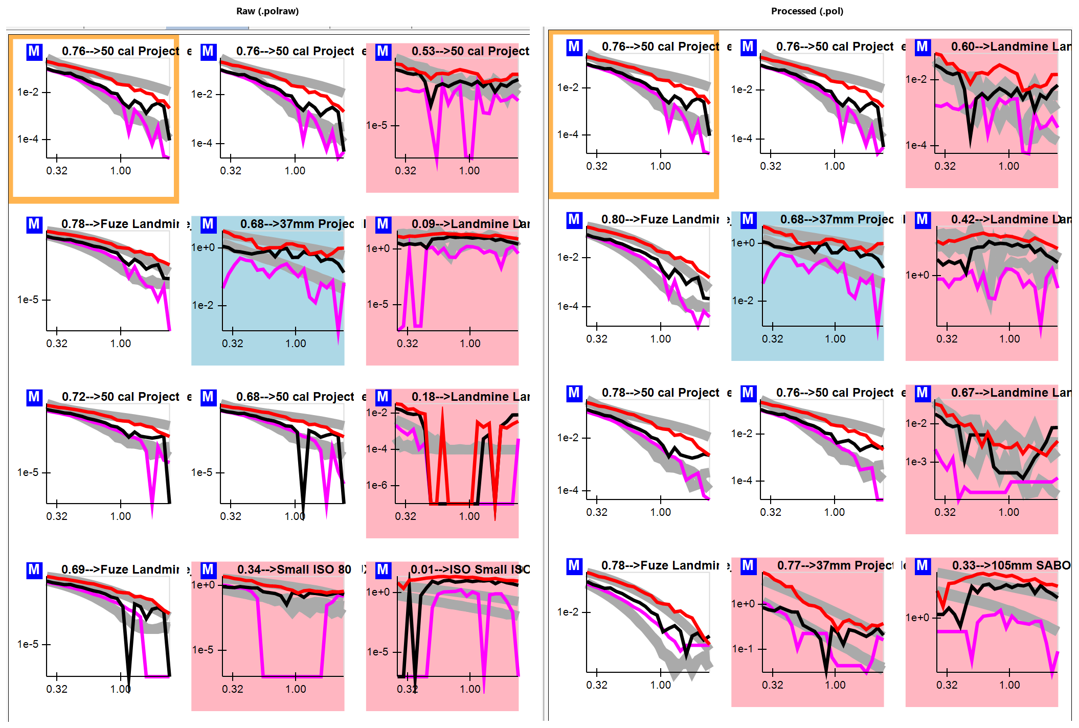
The effect of processing is easiest to see on the library-match plots, where the measured/predicted polarizability (magenta) is compared against the library curves. The raw curves (left) contain zero/negative gaps and isolated spikes that drop to the plot floor; after de-spiking, flooring and sorting, the processed curves (right) are smoother and match more consistently against the library.